Configuration Space of Robots
Contents
Table of Contents
▼
The configuration of a robot is a complete specification of the position of every point of the robot. The minimum number of real-valued coordinates needed to represent the configuration is the number of degrees of freedom (dof) of the robot.[*](Primary reference: Modern Robotics: Mechanics, Planning, and Control by Lynch & Park (2017). Northwestern University & Cambridge University Press.) The mathematical formalization of configuration space was first introduced by Lozano-Pérez in the context of robot motion planning (1983).[*](Historical context: T. Lozano-Pérez, "Spatial planning: a configuration space approach," IEEE Transactions on Computers (1983).)
The core relationship that allows us to use a minimal set of real-valued numbers is that rigid bodies have a fixed, known shape that never deforms. Because the object is rigid, the distance between any two points on its body remains absolutely constant regardless of where the object moves. If you were dealing with a soft or deformable object, like a pillow, the shape could change, and you would need an enormous number of variables to track the position of every shifting point to fully describe its state.
The -dimensional space containing all possible configurations of the robot is called the configuration space (C-space). At any given moment, the entire configuration of a robot can be represented simply as a single point within its C-space.
Consider a few concrete examples:
- A door: The physical configuration of a door requires only a single number to describe it: the angle about its hinge. Its C-space is 1-dimensional.
- A point on a plane: A point moving on a flat surface needs two coordinates, . Its C-space is a 2-dimensional plane.
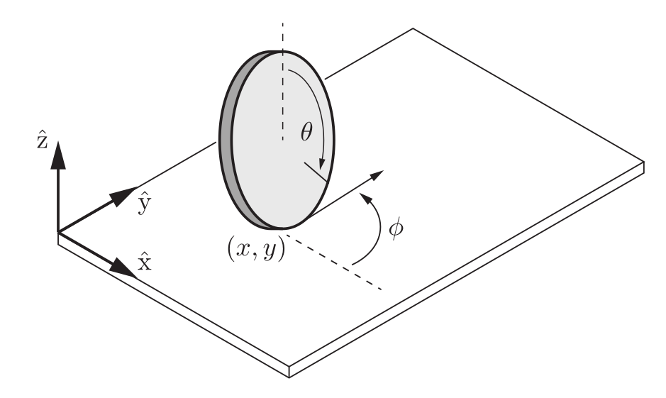
- A coin lying flat on a table: Described by three coordinates: for position and for orientation. Its C-space is 3-dimensional.
- A rigid body in 3D space: Requires six independent numbers ( position and three angles). Its C-space is 6-dimensional.
In essence, C-space allows us to translate the complicated physical motion of a multi-part robot into the simple mathematical motion of a single point moving through a high-dimensional space.
Robot Links
Robots are typically constructed from rigid bodies, called links, that are connected by various joints. Common joint types include revolute (hinge), prismatic (sliding), and spherical (ball-and-socket) joints, and each joint type provides specific freedoms while imposing constraints on the rigid bodies it connects.
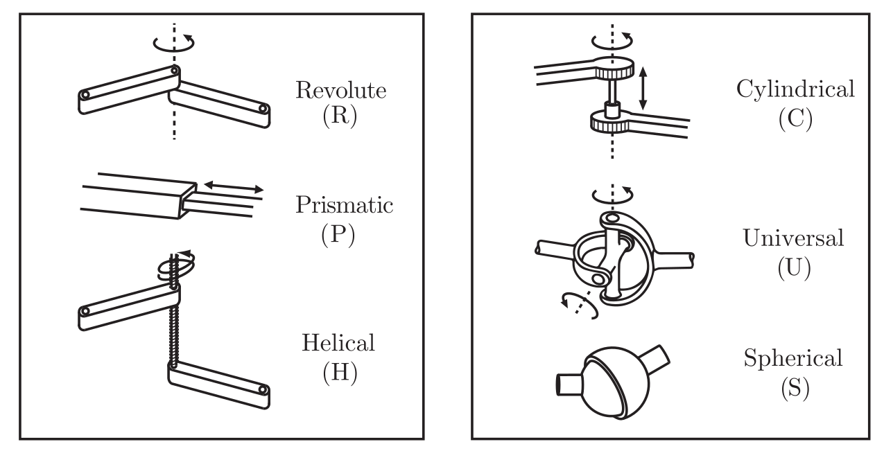
Robot Joint Types: Each joint type provides a specific number of freedoms while constraining all other relative motion.
Robot joints serve a dual purpose in defining a robot's configuration space: they provide specific freedoms of motion between rigid bodies while simultaneously acting as mathematical constraints that limit their overall movement. When two rigid bodies are connected by a joint, the total degrees of freedom of the system is reduced. The number of constraints a joint imposes, subtracted from the rigid body's inherent dof (three for a planar body and six for a spatial body), equals the exact number of freedoms that specific joint provides. This relationship is foundational for determining the dimension of a robot's overall C-space.
The following table identifies several typical robot joints, categorized by the number of freedoms they provide:
| DoF | Joint Name | Symbol | Motion Type |
|---|---|---|---|
| 1-DoF | Revolute (Hinge) | R | Pure rotation about a fixed axis. |
| Prismatic (Sliding) | P | Pure translation along a fixed axis. | |
| Helical (Screw) | H | Coupled rotation and translation along a screw axis. | |
| 2-DoF | Cylindrical | C | Independent translation and rotation about a single axis. |
| Universal | U | Pair of orthogonal revolute joints. | |
| 3-DoF | Spherical (Ball-and-Socket) | S | Three independent rotations, like a human shoulder. |
In the larger context of Configuration Space analysis, the specific types and quantities of joints are used to mathematically calculate the overall degrees of freedom of a robotic system using Grübler's formula.
Grübler's Formula
Grübler's formula is a mathematical tool used to precisely calculate the degrees of freedom (dof) of a robot, which directly defines the dimension of its configuration space (C-space).[*](Grübler's formula is also sometimes called the Chebychev–Grübler–Kutzbach criterion in the mechanism design literature.) In the broader kinematics literature, these systems are often referred to as mechanisms or linkages, and their mobility is a central subject of study.[*](Foundational mechanism analysis can be found in Erdman & Sandor (1996) and McCarthy & Soh (2011).) It formalizes the concept that a robot's overall C-space dimension equals the sum of the unconstrained freedoms of all its individual rigid bodies, minus the total independent constraints imposed by all connecting joints.
The formula uses the following variables:
- : Total number of links, counting the stationary ground as one link.
- : Total number of joints.
- : Baseline dof of a single rigid body ( for planar, for spatial mechanisms).
- : Number of independent freedoms provided by joint .
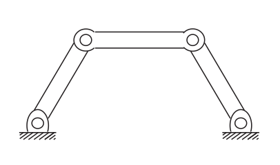
This equation works for both open-chain mechanisms (serial robotic arms) and closed-chain mechanisms (mechanisms with closed loops). However, there is a critical caveat: Grübler's formula strictly requires that all joint constraints within the system be completely independent. When redundant constraints are present, Grübler's formula only provides a lower bound on the actual number of degrees of freedom.
Short Quiz
A four-bar linkage has 4 links (including ground) and 4 revolute joints. Using Grübler's formula for a planar mechanism (m=3), what is its degree of freedom?
Topology and Representation
While degrees of freedom (dof) define the dimension of a robot's configuration space, the topology describes the fundamental shape of that space. Many robot C-spaces have the mathematical structure of a differentiable manifold, requiring tools from differential geometry to analyze correctly.[*](Accessible introductions to differential geometry for robotics include works by Millman & Parker (1977), do Carmo (1976), and Boothby (2002).) Two spaces are considered topologically equivalent if one can be continuously deformed into the other without any cutting or gluing.
For example, the surface of a sphere and a football are topologically equivalent because one can be stretched into the other, but a sphere cannot be deformed into a flat plane without being cut.
The topology of a complex robotic system can often be understood by expressing its C-space as the Cartesian product of simpler, lower-dimensional spaces:
- : -dimensional Euclidean space (e.g., a line or a plane ).
- : The -dimensional surface of a sphere in an -dimensional space (e.g., is a 1D circle).
- : An -dimensional torus, which is the product of circles ().
Using these building blocks, the C-space of a 2R robot arm (two revolute joints) is written as , which forms a torus (). Similarly, the C-space of a planar rigid body is , combining its 2D Euclidean translation with its 1D circular rotation.
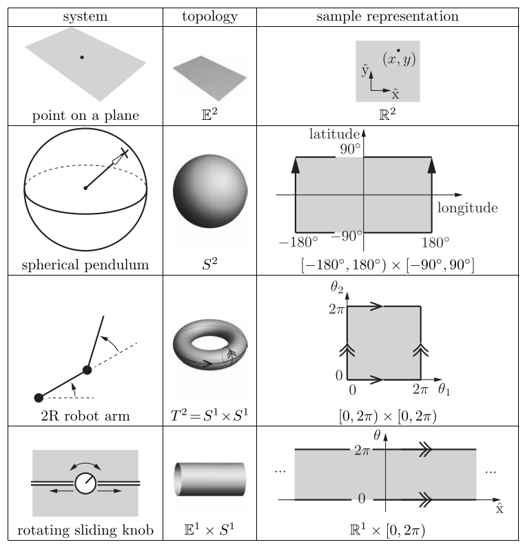
2R Robot C-space: The configuration space of a two-revolute-joint robot arm is topologically a torus .
Understanding topology is critical because if we ignore it and force a curved topological space into a flat grid of minimal coordinates (an explicit parameterization), we create mathematical singularities. A classic example is using latitude and longitude to map a sphere; this representation breaks down at the North and South Poles, causing velocity calculations to blow up toward infinity even when the robot's physical motion is smooth.
While topology is an inherent property of the space, representation is the subjective choice of numerical coordinates used to perform actual computations. This distinction is critical. If you use an explicit parameterization the absolute minimum number of coordinates to represent an -dimensional curved space, you will inevitably create singularities.
A classic example is using latitude and longitude (two coordinates) to represent a sphere (a 2D space). At the North and South Poles, the representation breaks down; taking a tiny physical step can result in an infinite rate of change in the longitude coordinate.
To overcome singularities, there are two representational strategies:
- An Atlas of Coordinate Charts: Uses multiple overlapping, explicitly parameterized "maps" that together cover the whole space. As the robot approaches a singularity on one chart, the system switches to an overlapping chart where the singularity does not exist. While this maintains the minimum number of coordinates, it requires complex bookkeeping.
- Implicit Representation: Views the -dimensional C-space as embedded inside a larger Euclidean space with dimensions (where ). It uses all coordinates, but restricts them using constraint equations.
For example, the 2D surface of a sphere () can be implicitly represented in 3D Euclidean space () using coordinates , subject to the constraint .
In the larger context of C-space analysis, implicit representation is overwhelmingly preferred despite using more numbers, because it completely eliminates singularities.[*](This is also why 3D rotation is standardly represented by a 9-number rotation matrix (subject to 6 constraints) rather than 3 Euler angles — it avoids singularities and easily supports standard linear algebra operations.) Furthermore, implicit representations are the natural mathematical framework for handling closed-chain robots, where the physical closed loops are modeled directly as implicit "loop-closure" constraint equations.
Constraints
Constraints are mathematical limitations placed on a system's motion, and they play a fundamental role in defining the dimension, representation, and behavior of a robot's C-space.
At the most basic level, the very definition of a rigid body relies on constraints: the distances between any points on the body must remain constant. When multiple rigid bodies are connected to build a robot, the joints act as physical constraints that restrict the independent movement of the connected links, thereby reducing the system's overall degrees of freedom. However, if a system possesses redundant constraints, Grübler's formula will only yield a lower bound on the true dimension of the C-space.
Constraints are divided into two major mathematical categories: configuration space constraints and velocity constraints. How these behave mathematically determines whether they fall into the category of holonomic or nonholonomic constraints.
Configuration Space Constraints (Holonomic)
Configuration constraints are physical restrictions that permanently tie the positions of a robot's links together. Because they directly limit where the robot can be, these constraints strictly reduce the dimension of the robot's C-space.
These constraints are expressed purely as position-level equations of the form:
where represents the configuration variables, and is a set of independent equations. Because they can be written as , all configuration constraints are inherently holonomic constraints.
When describing a point moving on the surface of a 3D sphere, we use an implicit representation by embedding the space into a higher-dimensional Euclidean space.
- Initial Coordinates (): We parameterize the point using 3 coordinates in , so .
- Constraints (): We apply a single distance constraint to ensure the point stays on the unit sphere: . Thus .
- Resulting C-space (): Applying this constraint restricts the valid configurations to a 2-dimensional surface () embedded in the 3D space. You have (r, ) to represent the space.
Velocity Constraints
Velocity constraints restrict the instantaneous directions a system can move, rather than tying its permanent coordinates together. They are mathematically referred to as Pfaffian constraints.
Velocity constraints are expressed as a matrix equation:
where is the joint-velocity vector, and is a matrix. Velocity constraints are subdivided into two kinds based entirely on whether they can be mathematically "integrated" into configuration constraints.
A. Integrable Velocity Constraints (Holonomic)
If a velocity constraint can be integrated to give an equivalent configuration constraint , it is considered holonomic. This means the velocity constraint is just a configuration constraint in disguise, and it successfully reduces the dimension of the C-space.
To see how this connects, suppose a robot follows a time trajectory subject to a configuration constraint . By differentiating both sides with respect to time, you get a velocity constraint:
Using the chain rule, this expands into a matrix multiplying the velocity vector:
This can be written compactly as:
Therefore, a Pfaffian constraint is holonomic if the matrix perfectly equals the partial derivative matrix for some function . In this case, is regarded as the integral of .
Imagine a tiny robot moving on a flat 2D floor with configuration variables . Tie the robot to a post at the origin with a rigid string of length .
The robot is forced to stay on a circle of radius , giving the configuration constraint:
Differentiating with respect to time gives the velocity constraint:
Putting this into matrix form :
To verify this is holonomic, we check whether . The partial derivatives of are exactly and — they match perfectly. Because we can mathematically "integrate" the velocity constraint back to the position constraint, the constraint is holonomic. The robot's C-space is permanently reduced from a 2D flat plane to a 1D circular line.
B. Nonintegrable Velocity Constraints (Nonholonomic)
If a velocity constraint cannot be integrated into a position-level equation, it is a nonholonomic constraint.[*](Nonholonomic constraints are central to mobile robotics. The kinematic constraints of wheeled vehicles and grasp contact kinematics both fall into this category.)
For a Pfaffian constraint , if there does not exist any differentiable function such that , the constraint is nonintegrable. Because they cannot be turned into equations, nonholonomic constraints strictly reduce the dimension of the system's feasible velocities, but they do not reduce the dimension of the reachable C-space.
A coin rolling upright on a plane without slipping. The "no-slip" velocity constraint restricts its instantaneous movement direction, but through maneuvering, the coin can still reach any configuration within its full 4-dimensional C-space.
Nonholonomic Constraint: A rolling coin cannot slip sideways instantaneously, yet it can maneuver to reach any in its 4D C-space.
Task Space and Workspace
Configuration space (C-space) represents the complete mathematical posture of every single joint and link of a robot. However, when analyzing what a robot is actually doing, engineers often utilize the concepts of task space and workspace, which both relate strictly to the configuration of the robot's end-effector rather than the entire machine.
Task Space is the space in which the robot's specific task can be naturally expressed.
- Driven by the Task: The mathematical definition of the task space is dictated entirely by the task itself, completely independent of the physical robot being used.
- Examples: If a robot's job is to plot with a pen on a flat piece of paper, its task space is a 2D plane (). If the task is to manipulate a rigid body in 3D space, the task space represents the 3D position and orientation of the end-effector. If the task is pointing a laser, the task space might simply be the spherical directions the laser can point (), because twisting the laser around its own beam axis does not change where the beam lands.
Workspace is a specification of the exact configurations that the robot's end-effector can physically reach.
- Driven by the Robot: Unlike task space, the workspace is dictated primarily by the robot's mechanical structure (its link lengths, joint limits, etc.), independently of whatever task it is assigned.
Summary
The configuration space (C-space) of a robot represents the set of all its possible physical postures, and its dimension is defined strictly by the robot's degrees of freedom (dof). Because a robot is constructed from rigid links connected by joints, its overall dof can be systematically computed using Grübler's formula, which balances the free mobility of the individual links against the mathematical constraints imposed by the joints.
To calculate movements safely, engineers must choose how to mathematically represent this C-space. Because curved topological spaces cause mathematical singularities when forced into flat, minimum-coordinate grids (explicit parameterization), it is standard to use an implicit representation. This method avoids singularities by using extra coordinates and restricting them with holonomic constraints — position-level equations that permanently tie variables together and successfully reduce the dimension of the actual reachable C-space. These are fundamentally different from nonholonomic constraints, which are velocity-level restrictions (like a wheel rolling without slipping) that limit instantaneous movement but do not shrink the robot's overall reachable space.
Finally, while C-space tracks the entire machine, a robot's practical application is evaluated using two end-effector concepts: the task space (the mathematical space naturally required to express a specific job) and the workspace (the physical space the robot's structure actually allows it to reach).