Decision Trees
Contents
Table of Contents
▼
Decision trees are versatile machine learning algorithms used for both classification and regression tasks. They are powerful algorithms, capable of fitting complex datasets and capturing nonlinear relationships. What sets decision trees apart is their interpretability—they are white box models, meaning their decisions are transparent and easily interpretable, unlike black box models like random forests and neural networks.[*](Primary reference: Hands-On Machine Learning with Scikit-Learn, Keras, and TensorFlow by Aurélien Géron (3rd edition, 2022).) This interpretability makes decision trees valuable in situations where understanding the reasoning behind predictions is important, such as medical diagnosis, credit scoring, and regulatory compliance.
How Decision Trees Work
Decision trees make predictions by navigating from the root node to a leaf node. Each node represents a decision based on a specific feature and threshold. The process starts at the root node and follows branches based on the feature values of the input instance until a leaf node is reached. The leaf node provides the predicted class (for classification) or value (for regression).
Visualizing Decision Trees
Decision trees can be visualized using the export_graphviz() function in Scikit-Learn, and the resulting output can be displayed using Graphviz.[*](Graphviz is an open-source graph visualization software package. See Graphviz documentation.) Graphviz is an open-source graph visualization software package that includes a command-line tool for converting .dot files to various formats, making it easy to visualize and understand the decision-making process of a trained tree.
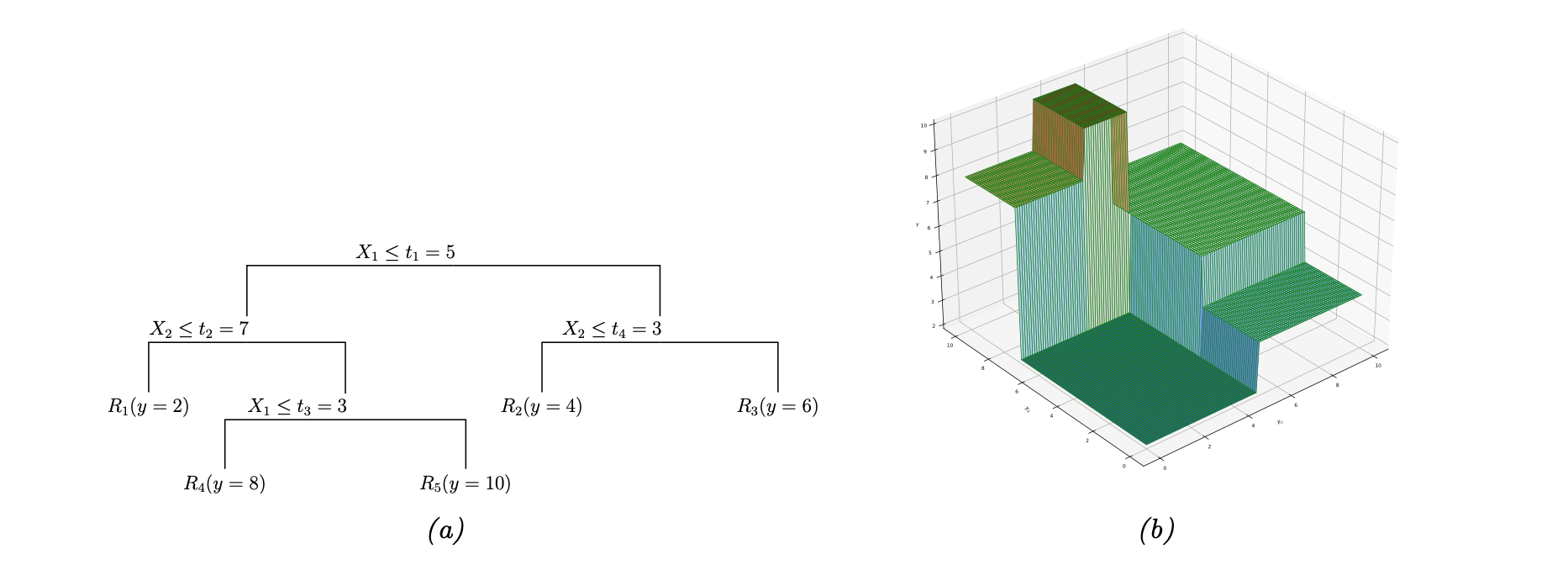
Decision Tree Visualization: A trained decision tree showing the path from root to leaf for making predictions on the iris dataset.
Making Predictions
For a new instance, the prediction process starts at the root node and follows the path based on the feature values and thresholds until a leaf node is reached. The leaf node gives the predicted class. Decision trees can also estimate class probabilities by calculating the proportion of training instances of each class in the corresponding leaf node.
Training Decision Trees: The CART Algorithm
Scikit-Learn employs the Classification and Regression Tree (CART) algorithm to train decision trees.[*](Algorithm reference: Classification and Regression Trees by Breiman, Friedman, Olshen, and Stone (1984).)
This algorithm recursively partitions the training set into subsets, aiming to minimize impurity for classification tasks and the mean squared error (MSE) for regression tasks.
The CART algorithm is a greedy algorithm, meaning it focuses on making the best split at each node without considering the overall impact on the tree's structure further down. While this simplifies the training process, it can lead to suboptimal trees that are highly sensitive to data variations.
Splitting Criteria: Gini Impurity and Entropy
The CART algorithm evaluates potential splits based on impurity measures like Gini impurity or entropy.[*](For more details on information theory and entropy, see Wikipedia: Entropy (Information Theory).)
Gini impurity of a node reflects the probability of misclassifying a randomly chosen instance from that node. A Gini impurity of 0 signifies a pure node where all instances belong to the same class.
In contrast, entropy, rooted in information theory, assesses the average information content needed to identify the class of an instance in a node. A node with zero entropy contains instances of only one class.
While both measures often lead to similar trees, Gini impurity is computationally faster, making it the default choice in Scikit-Learn. Entropy, however, tends to generate slightly more balanced trees, potentially leading to a more generalized model. Scikit-Learn allows selecting the impurity measure using the criterion hyperparameter in the DecisionTreeClassifier class.
Finding the Best Split
At each node, the algorithm evaluates all possible features and their thresholds to identify the split that yields the greatest reduction in impurity or MSE. The algorithm aims to create subsets that are as pure as possible.

Finding the Best Split: The CART algorithm evaluates all possible splits to minimize impurity at each node.
For instance, when training a DecisionTreeClassifier on the iris dataset, the algorithm might find that splitting based on petal length ≤ 2.45 cm results in the purest subsets.
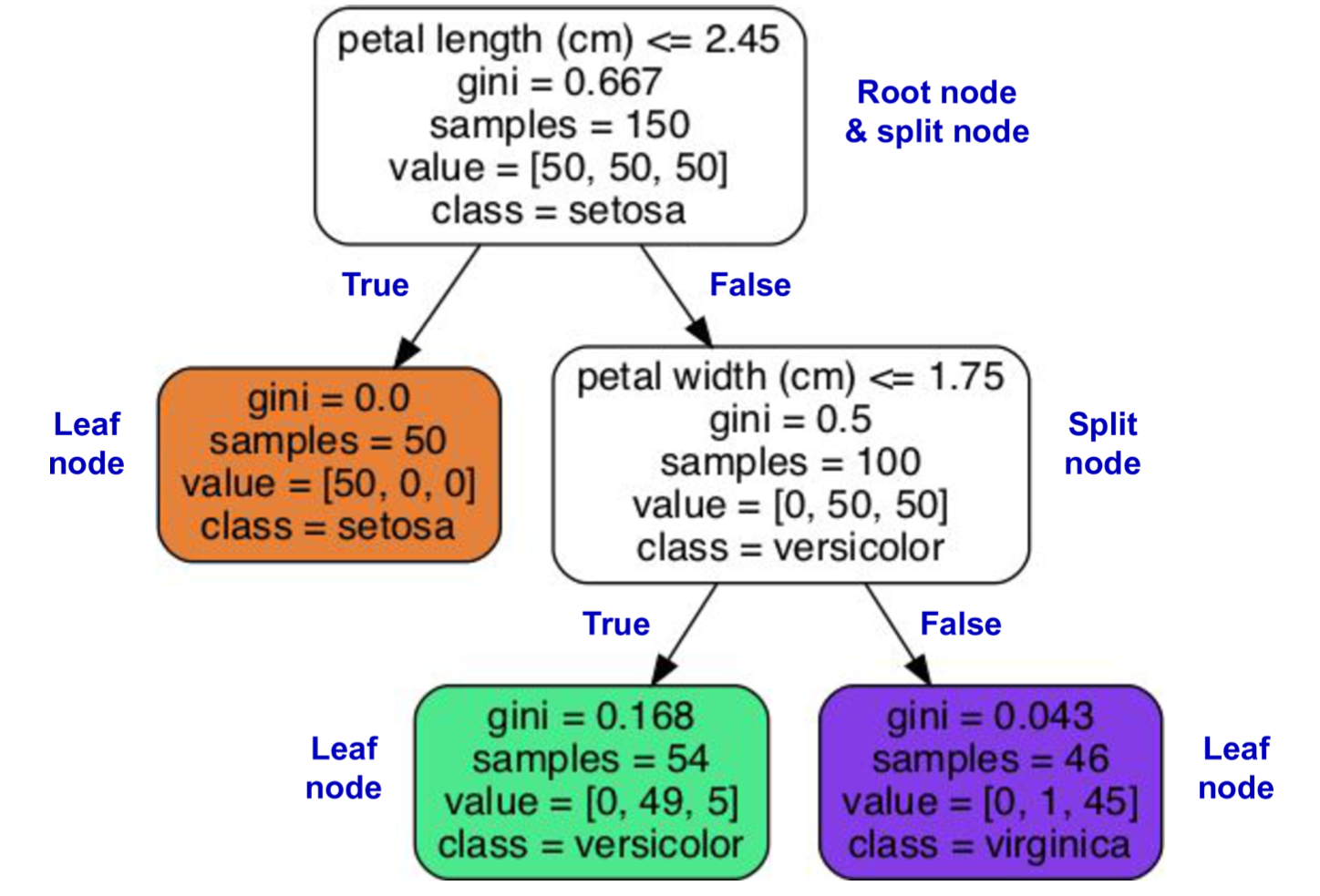
Iris Dataset Example: A decision tree trained on the iris dataset using petal length and width as features.
Recursive Splitting and Stopping Criteria
This process of splitting continues recursively, dividing the training set into increasingly homogeneous subsets. The recursion stops when specific criteria are met, such as reaching the maximum depth specified by the max_depth hyperparameter or encountering a node with fewer samples than min_samples_split.
Decision Trees for Classification and Regression
Decision trees can be used for both classification and regression tasks. For classification, each leaf node predicts a class label. For regression, each leaf node predicts a value, typically the average of the target values for the instances in that node.
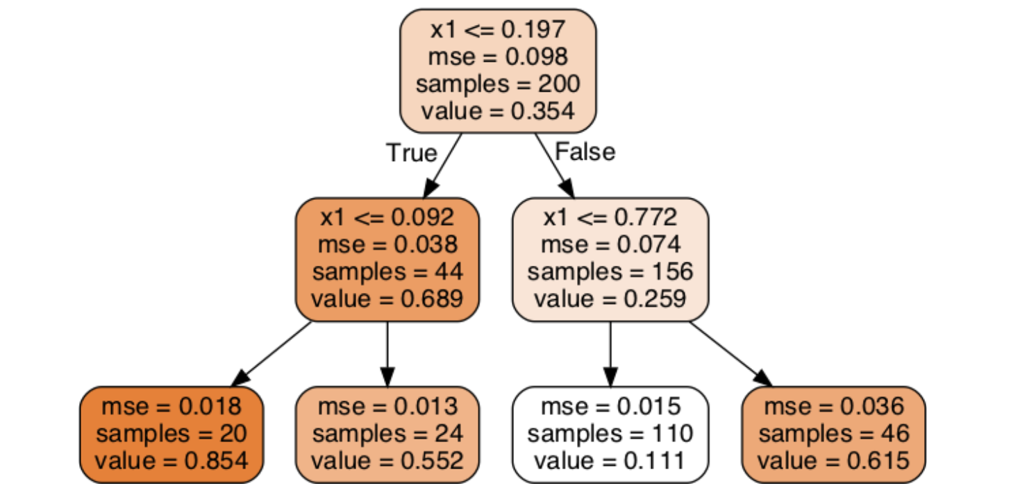
Regression Tree: A decision tree used for regression, where each leaf node predicts the average target value of instances in that region.
Cost Functions
The CART algorithm's objective is to minimize a cost function that quantifies the quality of a split. For classification, the cost function considers the impurity of the resulting subsets, weighted by their size. For regression, the cost function focuses on minimizing the MSE. The formulas for the cost functions are as follows:
Classification:
where:
- measures the impurity (Gini or entropy) of the left/right subset.
- is the number of instances in the left/right subset.
- is the total number of instances at the current node.
- is the feature index and is the threshold value.
Regression:
where:
- is the MSE of a node.
- is the average target value of instances in a node.
Example of CART in Action
Consider a regression tree example trained on a noisy quadratic dataset with max_depth=2. The tree splits the data based on thresholds for the input feature, predicting the average target value for instances within each resulting region. Increasing max_depth would lead to more splits and a more complex tree, potentially capturing the data's nonlinearity more accurately but also increasing the risk of overfitting.
Advantages and Disadvantages
Advantages
Decision trees offer several advantages:
| Aspect | Description |
|---|---|
| Easy to understand and interpret | The tree structure visually represents the decision-making process, making it easy to comprehend how predictions are derived. |
| Simple to use | They are relatively straightforward to implement and use, with libraries like Scikit-Learn providing convenient tools.[*](Scikit-Learn documentation: Decision Trees in Scikit-Learn.) |
| Versatile | They can handle both classification and regression tasks, accommodating various types of data. |
| Powerful | They are capable of fitting complex datasets and capturing nonlinear relationships. |
| Require very little data preparation | They do not require feature scaling or centering. |
| Perform automatic variable selection | The algorithm naturally selects the most informative features for splitting. |
| Relatively robust to outliers | Outliers typically affect only the leaf nodes they belong to. |
| Fast to fit, and scale well to large data sets | Modern implementations are highly optimized. |
| Can handle missing input features | Through techniques like surrogate splits (discussed later). |
| Insensitive to monotone transformations of the inputs | The algorithm only considers the ordering of feature values, not their absolute magnitudes. |
Disadvantages
Decision trees also have disadvantages:
| Aspect | Description |
|---|---|
| Sensitive to data orientation | They are sensitive to the orientation of the data and may create overly complex decision boundaries for rotated datasets. One way to mitigate this issue is to apply PCA to rotate the data in a way that reduces the correlation between features. |
| High variance | They can be prone to overfitting, meaning they may capture noise in the training data and not generalize well to new instances. Averaging predictions over multiple trees in an ensemble method like a random forest can reduce variance. |
| Instability | Small changes in the training data can lead to substantially different tree structures, as discussed in detail later. |
Regularization Techniques
Decision trees possess a remarkable ability to adapt to training data, often to the point of overfitting. Overfitting occurs when a model learns the training data too well, capturing noise and outliers that hinder its ability to generalize to unseen data. Regularization techniques are employed to curb a decision tree's flexibility during training, thus mitigating the risk of overfitting.
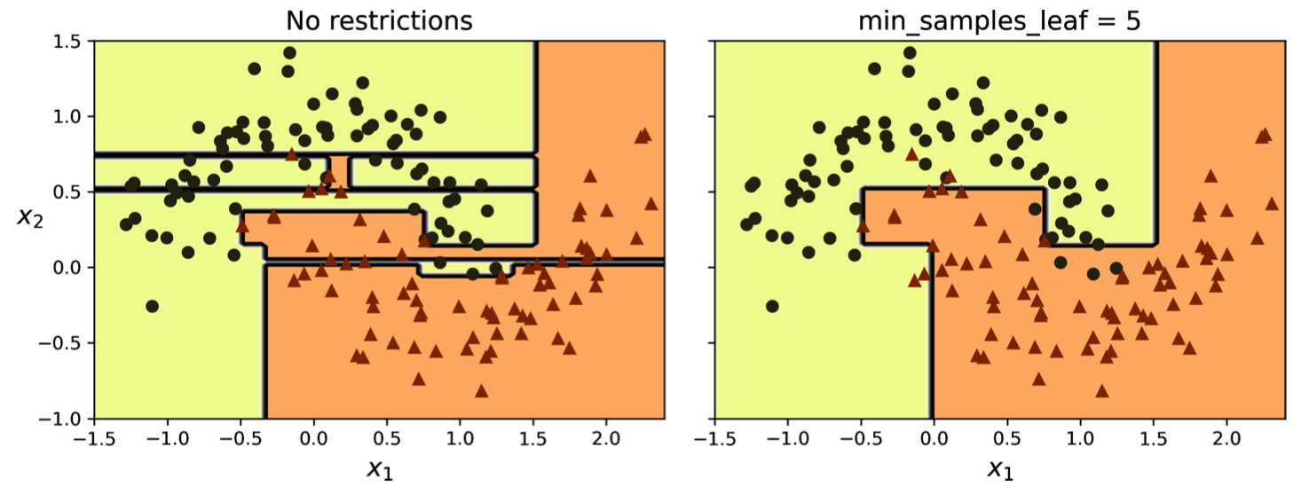
Overfitting Example: A decision tree that has overfit to the training data, creating overly complex decision boundaries.
Limiting the depth of a decision tree is a straightforward regularization method. Scikit-Learn provides the max_depth hyperparameter to control this aspect. A lower max_depth restricts the tree's growth, preventing it from becoming overly complex.
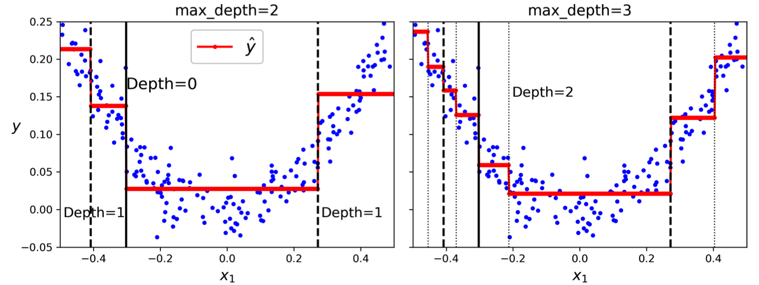
Regularized Tree: A decision tree with max_depth constraint, showing simpler decision boundaries that generalize better.
Scikit-Learn's DecisionTreeClassifier offers various hyperparameters to regulate the tree's structure:
max_features: Limits the number of features considered at each split. By evaluating a subset of features, the algorithm introduces randomness and reduces the tree's sensitivity to individual features, promoting generalization.max_leaf_nodes: Caps the number of leaf nodes in the tree. This constraint directly limits the tree's complexity and encourages the algorithm to focus on the most informative splits.min_samples_split: Sets the minimum number of samples required to split a node. Increasing this value prevents the algorithm from splitting nodes with too few samples, which could lead to overfitting.min_samples_leaf: Specifies the minimum number of samples a leaf node must have. This hyperparameter prevents the creation of leaf nodes with very few samples, again addressing the issue of overfitting.min_weight_fraction_leaf: Similar tomin_samples_leafbut expressed as a fraction of the total weighted instances. This option is particularly useful when dealing with weighted instances, allowing for more nuanced control over leaf node creation.
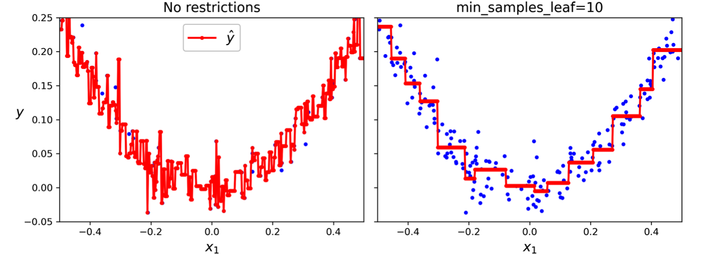
Regularization Effects: Comparison of decision boundaries with different regularization hyperparameter settings.
Increasing the values of hyperparameters starting with "min" or decreasing those starting with "max" generally results in a more regularized model. For example, increasing min_samples_leaf forces the tree to have more instances per leaf, leading to a simpler model less likely to overfit.
Challenges: Orientation Sensitivity and High Variance
Sensitivity to Axis Orientation
Decision trees exhibit a preference for orthogonal decision boundaries, making them susceptible to the orientation of the data. Orthogonal decision boundaries mean that splits are perpendicular to an axis, leading to a staircase-like pattern when visualizing the decision boundaries. This sensitivity arises because the CART algorithm evaluates splits based on individual features and their thresholds, without considering combinations of features or diagonal splits.
In its original orientation, a decision tree can easily separate the classes with a single, straight split. However, rotating the dataset by 45 degrees results in a more convoluted decision boundary with multiple orthogonal splits. While both trees might achieve perfect accuracy on the training data, the rotated tree is likely to generalize poorly to new data.
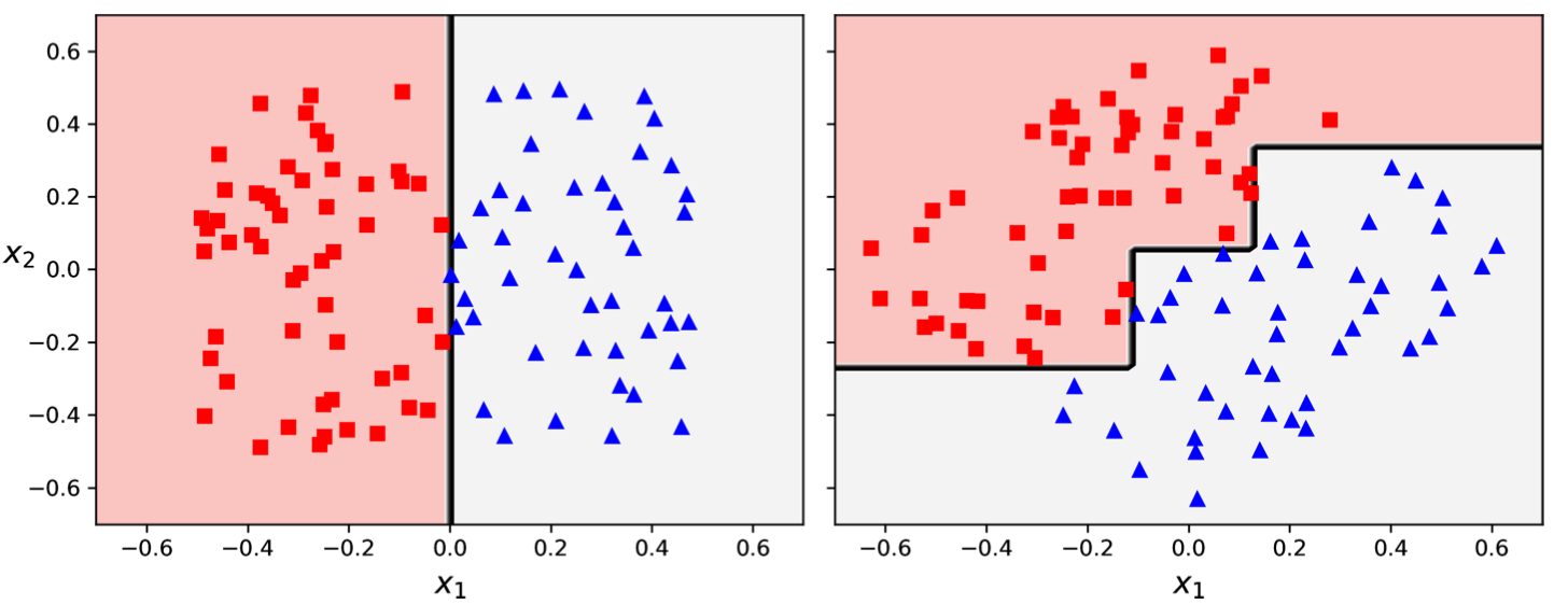
Orientation Sensitivity: The same dataset rotated by 45 degrees requires a more complex decision boundary with multiple splits.
Mitigating Sensitivity to Orientation: Feature Scaling and PCA
Feature scaling and Principal Component Analysis (PCA) can help alleviate this sensitivity to data orientation. Feature scaling ensures that all features have a similar range, preventing any single feature from dominating the splitting process. PCA, a dimensionality reduction technique, rotates the data to minimize the correlation between features.[*](For more on PCA, see the Wikipedia article on Principal Component Analysis.) This rotation can align the data with the axes, enabling the decision tree to make more effective splits.
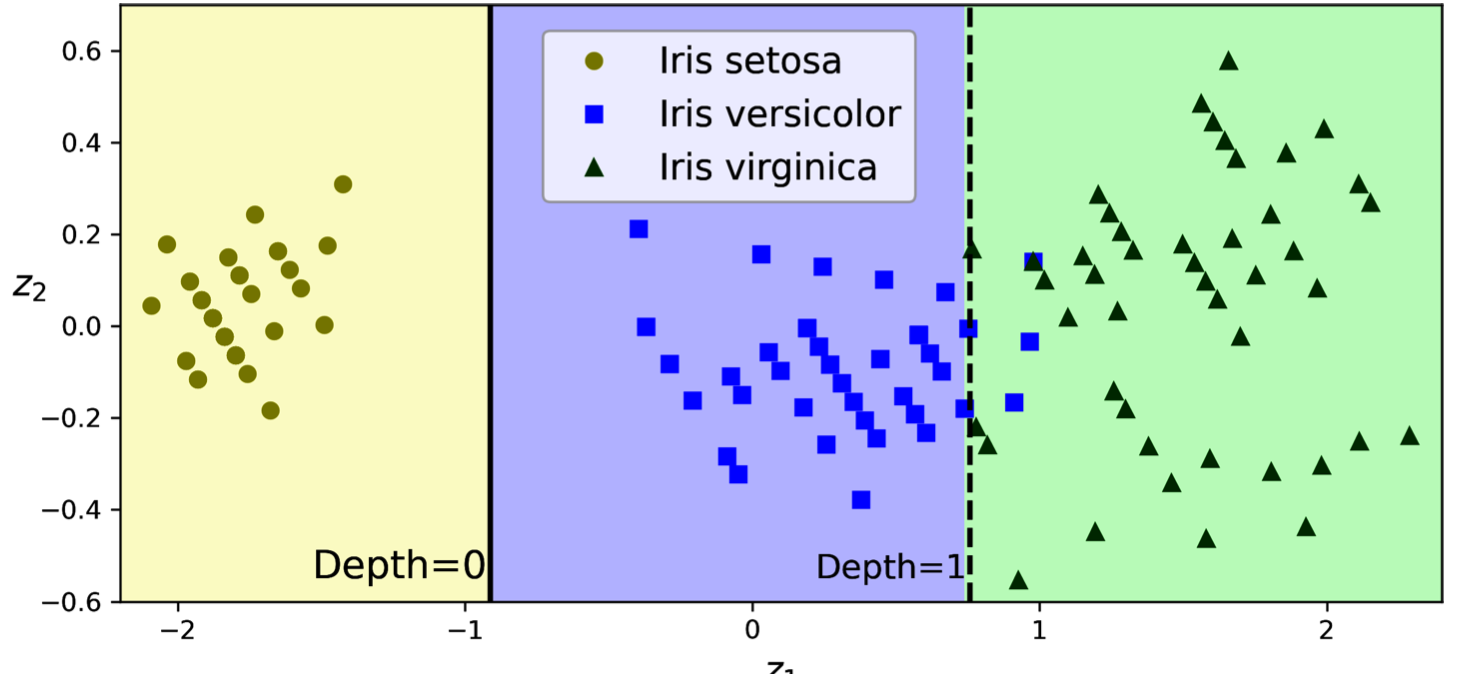
PCA Solution: Applying PCA to rotated data can help decision trees create more effective splits by aligning the data with the axes.
More on PCA here
Read More HereHigh Variance in Decision Trees
A significant limitation of decision trees is their high variance, meaning that small changes in the training data or hyperparameters can lead to substantially different models. This instability stems from the greedy nature of the CART algorithm and the hierarchical structure of decision trees. A slight change in a split near the root of the tree can cascade down, impacting subsequent splits and altering the entire tree structure.
Handling Missing Data
Decision trees can handle missing data through several strategies:
-
Surrogate Splits: When faced with missing data, decision trees can utilize surrogate splits. These are backup variables that create a similar data partition to the primary splitting variable when it's missing for a given instance. The process of finding surrogate splits involves identifying highly correlated features. If the primary splitting variable is unavailable, the algorithm uses the surrogate split to determine the appropriate branch.
-
Treating "Missing" as a Separate Category: For categorical variables, an alternative approach is to treat "missing" as a distinct category. This allows the algorithm to learn patterns associated with the missing values and make predictions accordingly.
The Instability of Decision Trees
Decision trees are inherently unstable, meaning that even small changes in the training data can significantly impact the tree's structure and lead to substantially different models.
This instability is a direct consequence of the hierarchical and greedy nature of the tree-building process, particularly the CART algorithm commonly used for training decision trees.
Reasons for Instability
Let's break down the reasons for this instability:
-
Hierarchical Structure: Decision trees make decisions in a hierarchical manner, starting from the root node and progressing down to the leaf nodes. Each split at a higher level of the tree determines the subsequent splits at lower levels. Consequently, even a slight change in a split near the root can cascade down, influencing all the subsequent splits and potentially altering the entire tree structure.
-
Greedy Splitting: The CART algorithm, a greedy approach, aims to find the best split at each node without considering the potential impact on future splits. It focuses on minimizing the impurity (for classification) or mean squared error (for regression) at the current node, without looking ahead to optimize the overall tree structure. This greedy behavior can lead to instability, as a slightly different split at a node might trigger a completely different set of splits in the subsequent levels.
-
Stochastic Nature of Feature Selection: When the
max_featureshyperparameter is explicitly set in Scikit-Learn'sDecisionTreeClassifier, the algorithm randomly selects a subset of features to evaluate at each node. By default, all features are considered at each split with no randomness. However, whenmax_featuresis set, this randomness introduces another layer of variability as retraining the same decision tree on the same data might result in a different set of features being chosen at each node, leading to a distinct tree structure. To ensure reproducibility, you can set therandom_statehyperparameter.
Visualizing Instability: An Example with the Iris Dataset
The iris dataset can be used to visually demonstrate the sensitivity of decision trees to data changes. A decision tree of depth 2 trained on the iris data, using only the petal length and petal width features, shows how the leaf nodes are color-coded based on the majority class, with the number of training samples reaching each node and their distribution across classes displayed.
Removing a single data point can dramatically alter the decision surface. The decision boundaries shift significantly due to the change in data, highlighting the instability of decision trees. This sensitivity makes individual decision trees prone to overfitting and can hinder their generalization performance on unseen data.
Overcoming Instability: Ensemble Methods like Random Forests
While the instability of decision trees poses a challenge, it's not an insurmountable one. Ensemble methods, particularly random forests, effectively address this issue by combining predictions from multiple decision trees.[*](For more on random forests, see Wikipedia: Random Forest.) Each tree in a random forest is trained on a random subset of the data and features, introducing diversity and reducing the impact of individual trees' variance. Averaging the predictions from these diverse trees results in a more stable and generalized model that is less susceptible to the instability of individual decision trees.
Conclusion
Decision trees are powerful, interpretable machine learning algorithms that excel in situations where understanding the reasoning behind predictions is crucial. Their white-box nature makes them valuable for applications requiring transparency, such as medical diagnosis, financial risk assessment, and regulatory compliance.
However, decision trees are not without their limitations. Their sensitivity to data orientation, high variance, and instability can make them challenging to use in isolation. The key to harnessing the power of decision trees lies in understanding these limitations and knowing when to use regularization techniques or ensemble methods like random forests to overcome them.
The CART algorithm's greedy, hierarchical approach makes decision trees fast to train and easy to interpret, but also contributes to their instability. By combining multiple trees through ensemble methods, we can leverage the strengths of decision trees—their interpretability and ability to capture complex patterns—while mitigating their weaknesses.
As we move forward in machine learning, the interpretability of decision trees remains valuable, even as we develop more complex models. Understanding how decision trees work provides a foundation for understanding ensemble methods and other advanced techniques that build upon these fundamental algorithms.