Embedding Compression via Spherical Coordinates

If you are building RAG (Retrieval-Augmented Generation) systems or working with Large Language Models, you know the "Embedding Tax." Storing millions of 1024-dimensional vectors is expensive (when you want better retrieval), and sending them over the internet is slow.

For a long while now, we've been stuck between two choices:

Lossy Compression (Product Quantization): Shrinks data a lot but hurts your retrieval accuracy. Used in quantizing models for low compute devices.

Standard Lossless Compression (Gzip/Zstd): Keeps accuracy perfect but barely manages a 1.2x shrink with reasons going to be apparent in the review blog.

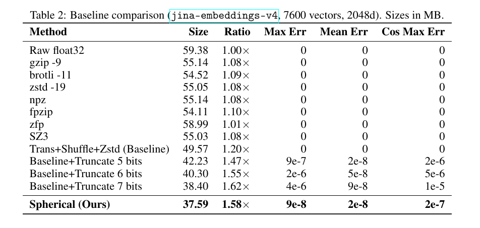
A recent paper by Han Xiao at Jina AI, titled "Embedding Compression via Spherical Coordinates,"[*](The original paper: Embedding Compression via Spherical Coordinates by Han Xiao (2025).) finally breaks this ceiling. By simply changing how we look at the math, they've achieved 1.5x lossless compression.

The Problem: Why Cartesian Vectors are Compression-Resistant

Most embedding models output vectors in Cartesian coordinates ($x, y, z \dots$). Because these models use Cosine Similarity, they normalize these vectors to a "unit-norm" (length = 1). Why? Because the industry standard for retrieval is Cosine Similarity [*](For a deep dive into vector normalization and its impact on search speed, see Embedding Quantization by Aarsen (2024).).

The formula for the cosine of the angle between two vectors $A$ and $B$ is $\text{sim}(A, B) = \frac{A \cdot B}{\|A\| \|B\|}$

By normalizing vectors to a length of 1 during training/inference, the denominator becomes $1 \times 1$. This turns a complex similarity calculation into a simple dot product, which is significantly faster for hardware like CPUs and GPUs to compute. The Geometric Consequence :If every vector has a length of 1, then every single embedding in your database lives on the surface of a hypersphere ($S^{d-1}$).

Here is the issue: to keep a vector's length at exactly 1.0 in Cartesian space, the individual numbers ($x, y, z$) have to vary wildly. One might be $0.003$ and the next might be $0.25$.

In the world of computer science and architecture, we store these as IEEE 754 32-bit floats. A float has three parts:

• Sign bit
• Exponent (The scale)
• Mantissa (The precision/fraction)

In Cartesian form, the Mantissa is high-entropy; it looks like random noise to a computer. Because it's "random," traditional algorithms like Zstd can't compress it. This is known as the 1.33x Wall[*](The "1.33x Wall" is a theoretical limit for float32 compression. Current SOTA methods like BitShuffle focus on grouping exponents but struggle with random mantissa bits.). Since the mantissa is 75% of the data and is uncompressible, you can never shrink the file by more than a tiny margin.

How Spherical Geometry Helps for Floating Number Compressions

The breakthrough in this paper is realizing that if all your vectors live on the surface of a sphere, you shouldn't be using $x, y, z$. You should be using angles.

The paper exploits a phenomenon called Geometric Concentration. In high-dimensional spaces (like a 1024-d embedding), the angles between vectors don't just go anywhere—they naturally cluster around $\pi/2$ (approximately 1.57). [*](This phenomenon is rooted in the law of large numbers for high-dimensional spheres. For the formal proof, see Distributions of angles in random packing on spheres by Cai et al. (2013).)

This has two massive benefits for compression:

1. Exponent Collapse: Because almost all the angles are near 1.57, their IEEE 754 Exponents become identical (value 127). Instead of storing thousands of different exponents, the compressor now sees the same bit pattern over and over. Entropy drops from 2.6 bits to nearly zero.
2. Mantissa Predictability: Because the values are so tightly clustered, even the "noisy" mantissa bits start to look the same. The first few bits of the fraction become predictable, dropping the mantissa entropy from a "random" 8.0 bits down to 4.5 bits.

By switching the "language" of the data from Cartesian to Spherical, we turn random noise into a highly patterned sequence that standard compressors can finally crush.

How it Works

The beauty of this method is that it's a "plug-and-play" pipeline. It follows a four-stage process to turn high-entropy Cartesian coordinates into low-entropy angular streams.

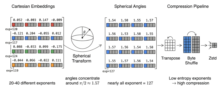
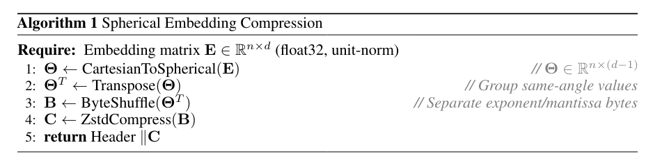
Step 1: The Spherical Transformation

We convert a $d$-dimensional Cartesian vector $x$ into $d-1$ angular coordinates $\theta$. Because $\|x\|_2=1$, the radius is always 1 and can be discarded, immediately reducing the data footprint by one dimension.

For the first $d-2$ angles, we use the inverse cosine of the current coordinate divided by the norm of the remaining coordinates: $\theta_i = \arccos \left( \frac{x_i}{\sqrt{\sum_{j=i}^d x_j^2}} \right), \quad i = 1, \dots, d-2$

For the final angle, we use the two-argument arctangent to preserve the full quadrant information of the hypersphere: $\theta_{d-1} = \operatorname{atan2}(x_d, x_{d-1})$ [*](Using $\operatorname{atan2}$ ensures the final angle maps to $[-\pi, \pi]$, covering the entire surface of the hypersphere, whereas $\arccos$ is limited to $[0, \pi]$.)

Step 2: Algorithmic Optimization (O(nd))

A naive calculation of the partial norms in the denominator would take $O(d^2)$ time, which is too slow for large embeddings. The paper optimizes this using backward cumulative summation. We precompute the squared norms from the end of the vector to the beginning: $r_i^2 = \sum_{j=i}^d x_j^2 = r_{i+1}^2 + x_i^2$ This allows the entire transformation to run in a single $O(d)$ pass, enabling the C implementation to exceed 1 GB/s throughput.

Step 3: Transposition and Byte Shuffling

If we have a batch of 1,000 vectors, we don't compress them individually. We lay them out in a matrix and transpose it. This groups the "Angle 1" of every vector together, then all the "Angle 2"s, etc.

Because of Measure Concentration, these angles are almost all near $1.5708$. In IEEE 754 float32, any number in the range $[1, 2)$ has an exponent of exactly 127. The result: After shuffling the bytes to group exponents together, the compressor sees a massive stream of identical 127 bytes, which compresses to nearly zero bits.

Step 4: Entropy Coding

Finally, the reordered byte stream is passed to Zstd. Because the "noise" (the mantissa) has been tamed by the geometric transform and the exponents have collapsed, Zstd can finally break the 1.33x wall.

Actual Python Implementation:[*](The transformation is mathematically invertible. Decompression simply applies the reverse trigonometric identities ($\sin$ and $\cos$) to reconstruct the Cartesian coordinates.)

import numpy as np
import zstandard as zstd

def compress(x, level=19): # x: (n, d) unit-norm float32
    n, d = x.shape
    xd = x.astype(np.float64) # Double precision for transforms
    ang = np.zeros((n, d-1), np.float64)
    for i in range(d-2):
        r = np.linalg.norm(xd[:, i:], axis=1)
        ang[:, i] = np.arccos(np.clip(xd[:, i] / r, -1, 1))
    ang[:, -1] = np.arctan2(xd[:, -1], xd[:, -2])
    ang = ang.astype(np.float32) # Store as float32
    shuf = np.frombuffer(ang.T.tobytes(), np.uint8).reshape(-1, 4).T.tobytes()
    return np.array([n, d], np.uint32).tobytes() + zstd.compress(shuf, level)

def decompress(blob):
    n, d = np.frombuffer(blob[:8], np.uint32)
    ang = np.frombuffer(zstd.decompress(blob[8:]), np.uint8).reshape(4, -1).T
    ang = np.frombuffer(ang.tobytes(), np.float32).reshape(d-1, n).T
    ang = ang.astype(np.float64) # Double precision for inverse
    x, s = np.zeros((n, d), np.float64), np.ones(n, np.float64)
    for i in range(d-2):
        x[:, i] = s * np.cos(ang[:, i])
        s *= np.sin(ang[:, i])
    x[:, -2], x[:, -1] = s * np.cos(ang[:, -1]), s * np.sin(ang[:, -1])
    return x.astype(np.float32)

Results and Real-World Impact

The results are stable across 26 different configurations. Whether you are using text, image, or multi-vector models, the 1.5x ratio holds firm.

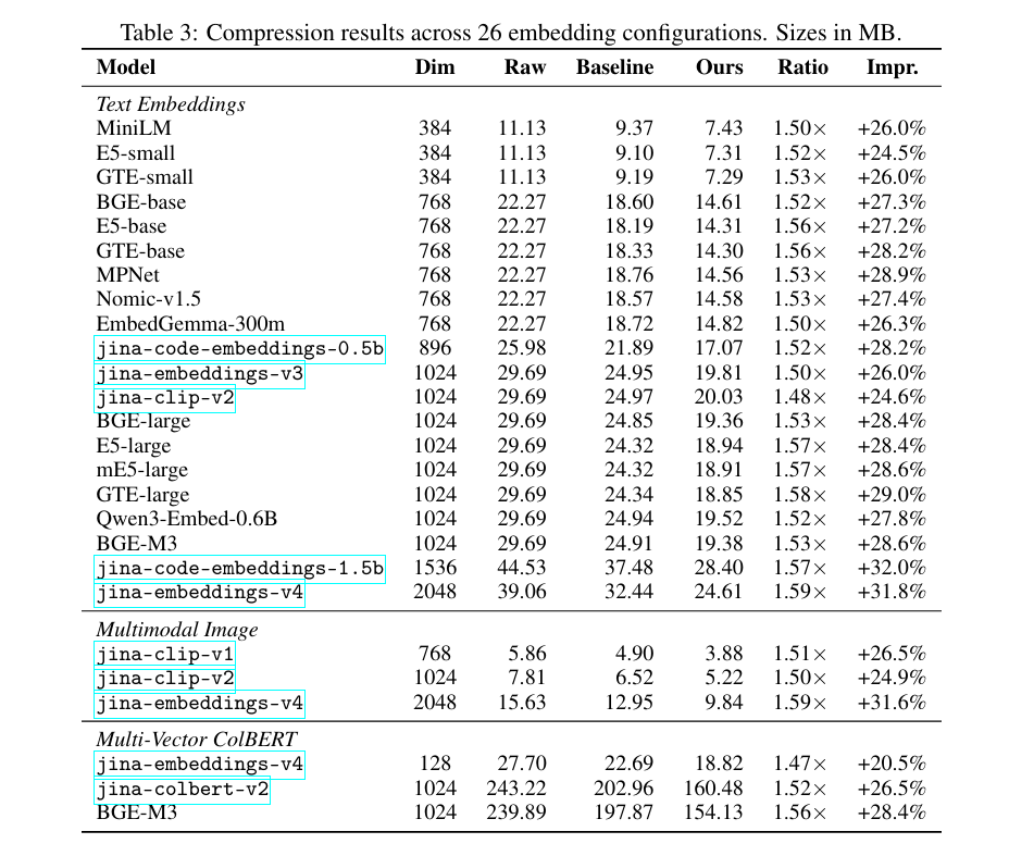
Why should you care?

If you are running a high-traffic embedding API or a massive vector database, this is a "free" win.

• Lower Latency: Sending 1.5x less data over HTTP means faster API responses.
• Lower Costs: 30% less storage means 30% lower database bills.
• Agility: Since it's training-free, you can implement this today on any model, from OpenAI's text-embedding-3-small to open-source BGE models.