Ensemble Learning
Contents
Table of Contents
▼
Ensemble learning is a machine learning technique that combines multiple individual models, often referred to as base models, to produce a more powerful and accurate predictive model.[*](Primary reference: Hands-On Machine Learning with Scikit-Learn, Keras, and TensorFlow by Aurélien Géron (3rd edition, 2022).) This strategy, inspired by the "wisdom of the crowd", leverages the principle that aggregating predictions from a group of models often yields better results than using the best individual model.
Ensemble learning is particularly effective when individual models exhibit high variance, meaning their predictions are sensitive to fluctuations in the training data. By combining multiple models, ensemble methods effectively reduce variance, resulting in more stable and generalized predictions. The success of ensemble methods in machine learning competitions, including the Netflix Prize, underscores their effectiveness and practical value in building high-performing predictive models.
Mathematical Foundations
Ensemble Model Formulation
Mathematically, an ensemble model can be represented as:
where:
- represents the ensemble model's prediction
- is the total number of base models in the ensemble
- represents the prediction of the th base model
This equation demonstrates how the ensemble model combines the predictions of individual base models. For regression tasks, the predictions are typically averaged. For classification tasks, a majority vote scheme can be used, where the class with the most votes from the base models is selected as the ensemble's prediction.
Suppose you build an ensemble containing 1,000 classifiers that are each correct only 51% of the time (barely better than random guessing). If you predict the majority class, you can hope for up to 75% accuracy! However, this is only true if all classifiers are perfectly independent, making uncorrelated errors, which is clearly not the case since they are trained on the same data. They are likely to make the same types of errors, so there will be many majority votes for the wrong class, reducing the ensemble’s accuracy.
To understand the effectiveness of ensemble learning, consider an ensemble of binary classifiers, each with an accuracy of . Assuming the correct class is 1, let:
- represent the prediction of the th model
- represent the total number of votes for class 1
The ensemble's prediction is determined by majority vote:
- Class 1 is predicted if
- Class 0 is predicted otherwise
The probability () that the ensemble will correctly predict class 1 is:
where:
- is the cumulative distribution function (CDF) of the binomial distribution with parameters and , evaluated at
This example illustrates how an ensemble of even slightly better-than-random classifiers () can achieve high accuracy when the ensemble size () is sufficiently large, assuming the errors made by individual classifiers are independent.
Voting Classifiers
Voting classifiers are a straightforward yet powerful ensemble method that leverages the principle of "wisdom of the crowd" to make predictions. Instead of relying on a single classifier, a voting classifier aggregates the predictions of multiple individual classifiers to arrive at a final prediction. The class that receives the most votes from the individual classifiers is chosen as the ensemble's prediction.
This approach can be likened to seeking opinions from multiple experts and choosing the most popular opinion as the final decision.
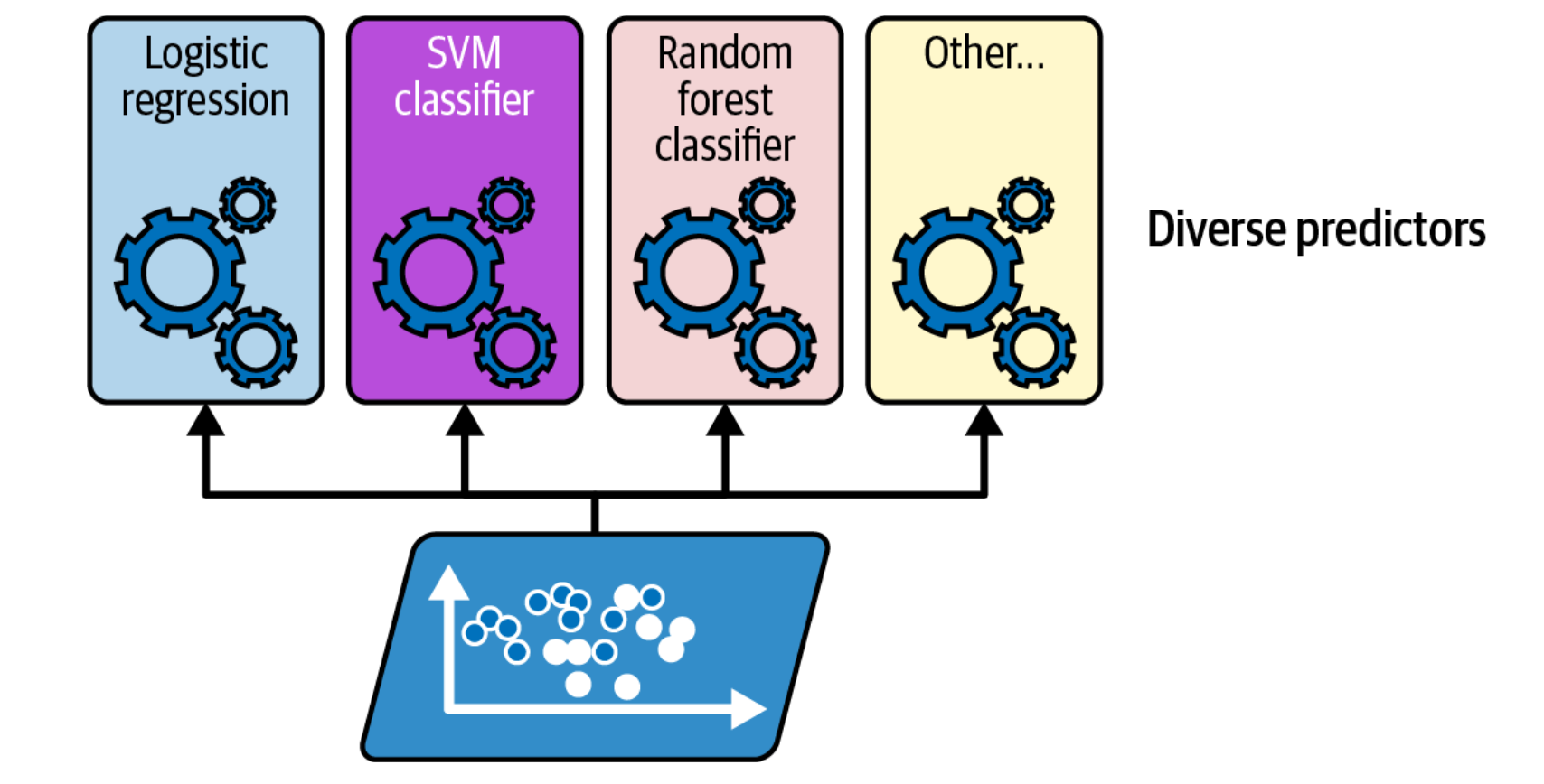
Voting Classifier: Multiple base models make predictions, and the ensemble selects the class with the majority of votes.
Hard Voting vs. Soft Voting
There are two main types of voting classifiers: hard voting and soft voting.
Hard voting classifiers simply count the votes of each individual classifier for each class, and the class with the majority of votes wins. This is analogous to a democratic voting system.
Soft voting, on the other hand, takes into account the confidence level of each classifier's prediction. Instead of just counting votes, soft voting averages the probabilities that each classifier assigns to each class. The class with the highest average probability is then chosen as the ensemble's prediction. This method is often more accurate than hard voting, as it gives more weight to the predictions of classifiers that are highly confident.
Key Considerations for Voting Classifiers
Diversity of Base Models: For a voting classifier to be effective, the individual classifiers should be diverse. This means they should use different algorithms, have different strengths and weaknesses, and make different types of errors. If the base models are too similar, the voting classifier will not perform much better than any of the individual classifiers.
Soft vs. Hard Voting: If all of your base classifiers are able to estimate class probabilities, then you should use soft voting, as it often achieves higher performance than hard voting.
Computational Cost: The computational cost of a voting classifier is generally the sum of the computational costs of the individual classifiers. This can be a significant overhead if you have many classifiers or if the individual classifiers are computationally expensive.
To use a voting classifier, you need to train multiple individual classifiers on the same training data. It is important to select diverse classifiers that use different algorithms. This helps to ensure that the classifiers will make different types of errors, which improves the ensemble's accuracy. For example, you might combine a logistic regression classifier, a support vector machine classifier, and a random forest classifier.
Bagging and Pasting
Bagging and pasting are ensemble methods that focus on creating diversity among base models by training them on different subsets of the training data. Both techniques employ the same learning algorithm for each model, but they differ in how they sample the training data:
-
Bagging (Bootstrap Aggregating): In bagging, random subsets of the training data are created by sampling with replacement. This means that the same instance can be selected multiple times for a given subset.
-
Pasting: Pasting creates random subsets of the training data by sampling without replacement. Each instance can only be selected once for a particular subset.
Understanding Bootstrap Sampling
The disadvantage of bootstrap sampling is that each base model only sees, on average, 63% of the unique input examples. To see why, note that the chance that a single item will not be selected from a set of size in any of draws is . In the limit of large , this becomes , which means only of the data points will be selected.
Rationale and Benefits
By training base models on different subsets of the data, bagging and pasting introduce variability in the learning process, leading to models that make different types of errors. This diversity in predictions ultimately reduces the variance of the ensemble model, resulting in improved generalization performance.
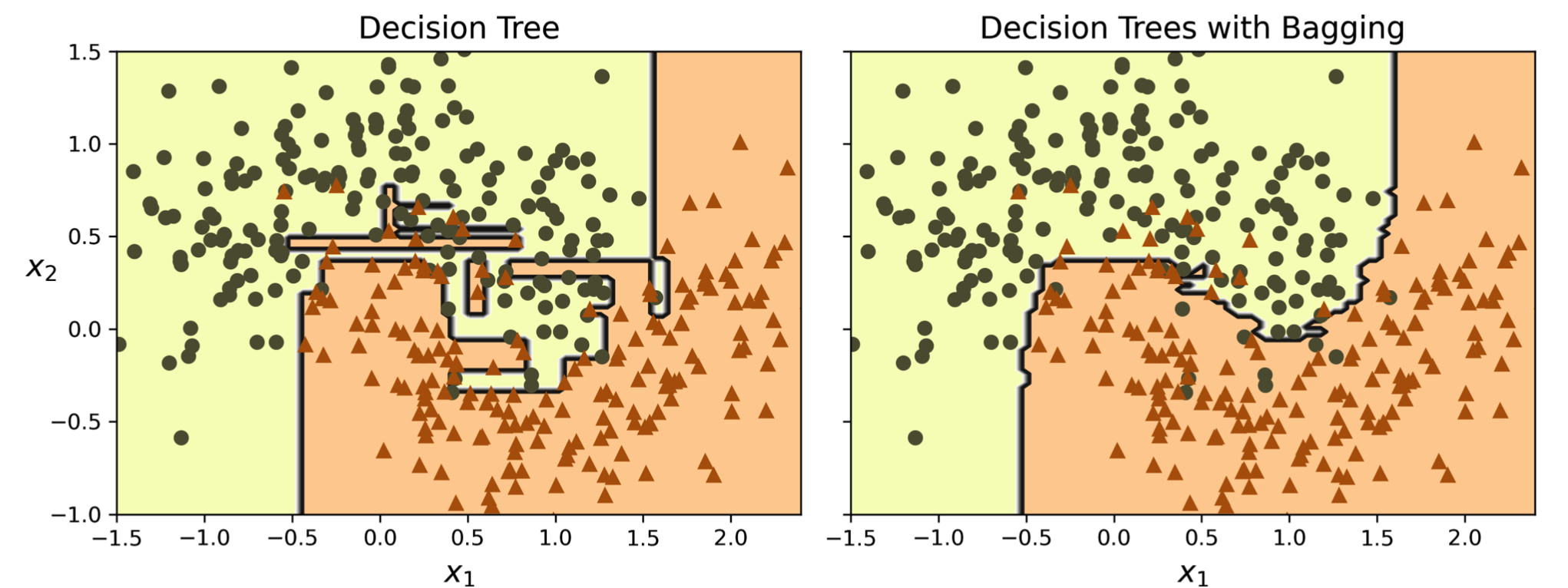
Bagging and Pasting: Training multiple models on different subsets of data to create diversity and reduce variance.
Bagging vs. Pasting
While both methods promote model diversity, bagging typically results in slightly higher bias compared to pasting. This is because the random sampling with replacement in bagging introduces some level of redundancy in the training subsets. However, this extra diversity also leads to lower correlation among the predictors, further reducing the ensemble's variance. In practice, bagging often outperforms pasting due to its superior variance reduction capabilities.
Out-of-Bag Evaluation
A unique characteristic of bagging is the concept of out-of-bag (OOB) evaluation. Due to the sampling with replacement in bagging, on average, only about 63% of the unique training instances are used to train each base model. The remaining 37% of the instances, not included in a particular model's training subset, constitute the OOB instances.
The OOB instances can be utilized to estimate the generalization performance of the ensemble without the need for a separate validation set. By evaluating each base model on its corresponding OOB instances and averaging the results, we obtain an OOB score, which serves as a measure of the ensemble's performance.
Key Advantages of Bagging and Pasting:
- Enhanced Generalization: Bagging and pasting effectively reduce variance, improving the ability of the ensemble model to generalize to unseen data.
- Parallelization: The training and prediction processes in bagging and pasting can be easily parallelized, enabling efficient training on large datasets.
- Out-of-Bag Evaluation: Bagging offers a convenient and computationally efficient way to estimate model performance using OOB evaluation, reducing the need for cross-validation.
Applications:
Bagging and pasting are particularly effective when used with unstable learning algorithms, such as decision trees. They are widely employed in various ensemble methods, including random forests and some variations of boosting algorithms.
Random Forests
Random Forests are a powerful ensemble learning method that builds upon the concept of bagging with decision trees.[*](Original paper: Random Forests by Breiman (2001).) They combine the predictions of multiple decision trees to create a robust and accurate model.
Random Forests address some limitations of individual decision trees, primarily their tendency to overfit, by combining multiple trees into an ensemble. The sources highlight two main techniques for creating this ensemble: bagging and random subspace method.
Bagging (Bootstrap Aggregating)
Bagging involves training each decision tree in the ensemble on a different random subset of the training data. These subsets are created by sampling with replacement, meaning that some instances might be selected multiple times for a single tree while others might be excluded.
Random Subspace Method
The random subspace method, employed in Random Forests, introduces further randomness by selecting a random subset of features for each node during tree construction. This forces trees to focus on different aspects of the data, further promoting diversity and reducing correlation among individual trees.
Extremely Randomized Trees (Extra-Trees)
Extra-Trees take the randomization a step further by not only selecting random subsets of features but also picking random thresholds for each feature at every node.[*](For more on Extra-Trees, see Wikipedia: Extremely Randomized Tree.) This additional randomness leads to even faster training times compared to regular Random Forests, as finding the best threshold for each feature is a computationally intensive task.
Advantages of Random Forests
| Aspect | Description |
|---|---|
| High Accuracy | Random Forests consistently achieve high accuracy on a wide range of tasks, often outperforming individual decision trees and other learning algorithms. |
| Robustness | Random Forests exhibit robustness to noisy data and outliers due to the averaging effect of multiple trees. |
| Feature Importance | Random Forests offer a built-in mechanism to assess the importance of features, providing insights into the data and facilitating feature selection. |
| Scalability | Random Forests can be trained efficiently in parallel, making them suitable for handling large datasets. |
Mathematical Justification: Bias-Variance Trade-off
The effectiveness of ensemble methods like Random Forests can be understood through the lens of the bias-variance trade-off.
- Bias: Bias refers to the error introduced by approximating a real-world problem with a simplified model.
- Variance: Variance represents the model's sensitivity to fluctuations in the training data. High variance models tend to overfit, performing well on the training data but poorly on unseen data.
Ensemble methods like Random Forests aim to reduce variance by averaging the predictions of multiple models. While individual trees might have high variance, the ensemble's prediction is less sensitive to the specific training data used for each tree.
Feature Importance: A Mathematical Perspective
Random Forests provide a valuable tool for assessing the relative importance of each feature in the dataset.
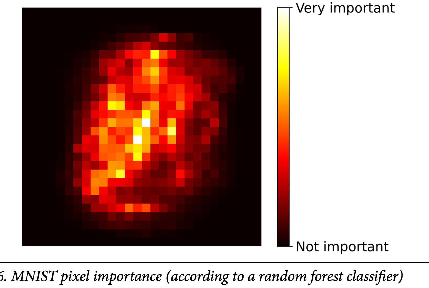
Feature Importance: Random Forests can assess the relative importance of features based on how much they reduce impurity across all trees.
The sources describe a method for calculating feature importance based on how much the tree nodes using a particular feature reduce impurity. For a single decision tree, the importance of feature is given by:
where:
- The sum is over all non-leaf nodes
- represents the gain in accuracy (reduction in cost) at node
- if node uses feature
- is an indicator function equal to 1 when node uses feature
To obtain a more stable estimate, the importance is averaged over all trees in the ensemble:
These scores are then scaled to ensure the sum of all importances equals 100%.
Boosting
Boosting is another powerful ensemble learning technique that combines multiple weak learners to create a strong learner, often achieving higher accuracy than any individual learner.[*](Original AdaBoost paper: A Decision-Theoretic Generalization of On-Line Learning and an Application to Boosting by Freund & Schapire (1997).) Boosting sequentially trains the models, where each model attempts to correct the errors of its predecessors. This process focuses on the harder examples, gradually improving the ensemble's performance.
AdaBoost: Adaptively Weighting Misclassifications
Core Concept and Algorithm
AdaBoost (Adaptive Boosting) is an algorithm that iteratively trains a series of weak learners, typically decision trees, by adjusting the weights of the training instances. The algorithm focuses on instances misclassified by previous learners. Let's break down the process step-by-step:
-
Initialization: Initially, all training instances are assigned equal weights (, where is the number of instances).
-
Iterative Training: For each iteration (, where is the number of learners):
-
Train a weak learner: A base classifier, , is trained using the current instance weights.
-
Calculate the weighted error rate: The error rate () of the learner is determined by the sum of weights of misclassified instances:
-
where is an indicator function, equal to 1 if the instance is misclassified and 0 otherwise.
- Compute the learner's weight: The weight () of the learner reflects its performance:
The learning rate, (typically set to 1), controls the contribution of each learner.
- Update instance weights: The weights of misclassified instances are increased, while the weights of correctly classified instances are decreased:
These weights are then normalized to ensure they sum up to 1.
- Ensemble Prediction: The final prediction for a new instance is obtained by weighted voting of all the learners:
Intuition and Visualization
The sources illustrate the process of AdaBoost with visualizations showing the sequential training process and how instance weights are updated. The decision boundaries of consecutive learners demonstrate how the ensemble progressively focuses on the harder instances, effectively reducing the error.
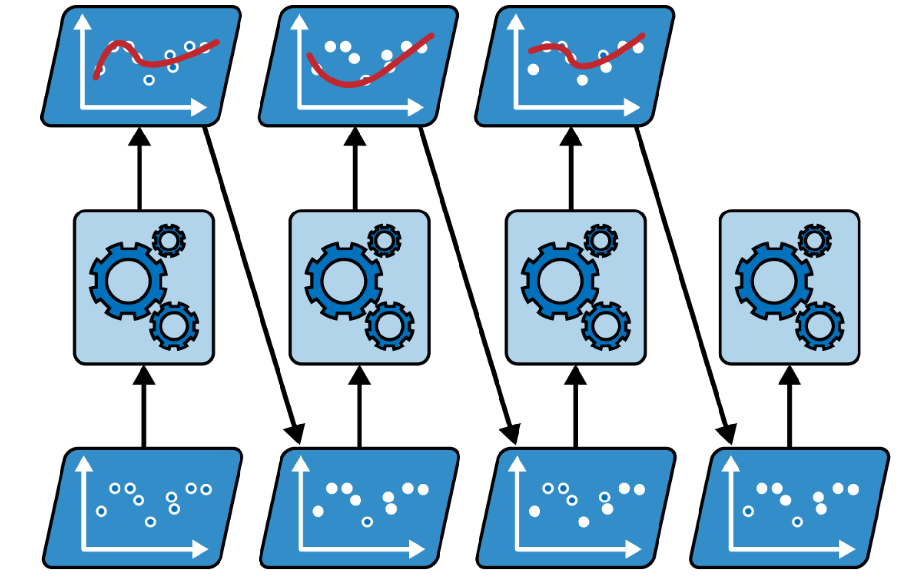
AdaBoost Training: Sequential training process showing how instance weights are updated to focus on misclassified examples.
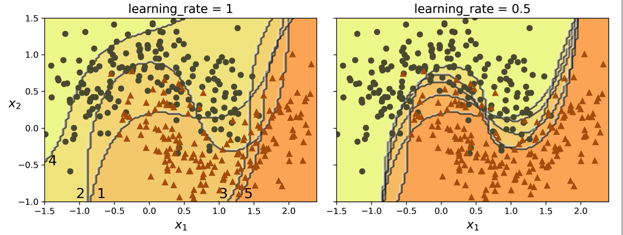
AdaBoost Decision Boundaries: How consecutive learners progressively focus on harder instances, improving the ensemble's accuracy.
Advantages and Limitations
| Aspect | Description |
|---|---|
| High accuracy | AdaBoost often achieves significant improvements in accuracy over individual weak learners. |
| Simplicity | The algorithm is relatively straightforward to implement and understand. |
| Sensitivity to outliers | AdaBoost can be sensitive to noisy data and outliers, as they can heavily influence the weights of subsequent learners. |
| Sequential training | The training process is inherently sequential, hindering parallelization and scalability for very large datasets. |
Gradient Boosting: Minimizing Loss Through Gradient Descent
A General Framework
Gradient Boosting is a more generalized boosting approach that can be used for both classification and regression tasks. Instead of adjusting weights of instances, Gradient Boosting focuses on minimizing a chosen loss function by iteratively adding weak learners to the ensemble. The key principle is to fit each new learner to the negative gradient of the loss function with respect to the current ensemble's predictions.
Algorithm Overview
The sources outline the following steps for Gradient Boosting:

Gradient Boosting Algorithm: Overview of the iterative process for building a gradient boosted ensemble.
-
Initialize the ensemble: The ensemble is often initialized with a simple model that minimizes the loss function on the training data.
-
Iterative Training: For each iteration :
- Compute the negative gradient: Calculate the negative gradient of the loss function () with respect to the ensemble's current prediction () for each instance :
-
Fit a weak learner to the gradient: Train a weak learner, , to predict the negative gradient ().
-
Update the ensemble: Add the new learner to the ensemble, scaled by a learning rate ():
- Ensemble Prediction: The final prediction is made by combining the predictions of all learners in the ensemble.
Loss Functions and Variants
The choice of loss function depends on the specific task. For regression, the squared error loss is commonly used. For classification, the log loss (also known as cross-entropy) is often preferred. The sources mention several variants of Gradient Boosting:
- Gradient Tree Boosting (GBRT): Uses decision trees as the weak learners. The sources provide an example of GBRT for regression, demonstrating how each tree fits the residual errors of the previous ensemble.
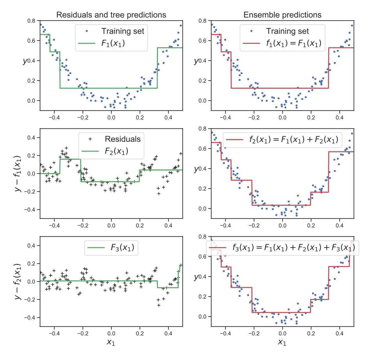
Gradient Tree Boosting: Visualization showing how each tree fits the residual errors of the previous ensemble, progressively improving predictions.
-
Stochastic Gradient Boosting: Introduces randomness by training each tree on a random subset of the training data.
-
Histogram-Based Gradient Boosting (HGB): Improves efficiency by binning the input features, making it suitable for large datasets.
Advantages and Limitations
| Aspect | Description |
|---|---|
| High accuracy | Often considered one of the most powerful machine learning algorithms. |
| Flexibility | Can handle various loss functions and types of weak learners. |
| Feature importance | Provides insights into the importance of features. |
| Computational cost | Can be computationally expensive, especially for large datasets and complex models. |
| Risk of overfitting | Requires careful tuning of hyperparameters to prevent overfitting. |
| Sequential training | Like AdaBoost, the training process is sequential, limiting parallelization. |
XGBoost: Extreme Gradient Boosting
The sources mention XGBoost (Extreme Gradient Boosting) as a highly optimized implementation of Gradient Boosting, known for its efficiency and performance.[*](XGBoost paper: XGBoost: A Scalable Tree Boosting System by Chen & Guestrin (2016).) XGBoost incorporates several enhancements, including:
- Regularization: Adds a penalty term to the loss function to control model complexity.
- Second-order optimization: Uses a second-order approximation of the loss function for potentially faster convergence.
- Feature subsampling: Randomly selects a subset of features at each node, similar to Random Forests.
- Scalability: Employs various techniques to handle large datasets and utilize computational resources efficiently.
The Mathematics Behind XGBoost
XGBoost is an optimized implementation of gradient boosted trees that enhances performance and efficiency. The sources provide a mathematical breakdown of XGBoost, including its regularized objective function, second-order approximation of the loss, and greedy optimization strategy.
Regularized Objective Function
XGBoost optimizes a regularized objective function that combines the loss function with a regularization term. This regularization term helps control the complexity of the model and prevents overfitting. The objective function is given by:
where:
- is the loss function measuring the difference between the true label () and the predicted output () for instance
- is the regularization term, defined as:
Here:
- is the number of leaves in the tree
- and are regularization coefficients controlling the strength of regularization
- represents the weight of the th leaf
Second-Order Approximation
XGBoost uses a second-order Taylor expansion to approximate the loss function at each step. This approximation allows for potentially faster convergence compared to using only a first-order approximation. The second-order approximation of the loss function at step is:
where:
- is the first derivative of the loss function with respect to evaluated at (the gradient)
- is the second derivative of the loss function (the Hessian)
Tree Structure and Weight Optimization
XGBoost uses regression trees as weak learners. Each tree partitions the data into regions based on feature values, and each region is assigned a weight. The tree structure and weights are optimized using a greedy approach to build the tree structure, starting with a single leaf and recursively splitting nodes to minimize the loss. Once the tree structure is determined, XGBoost finds the optimal leaf weights by minimizing the approximated loss function.
Stacking: Meta-Learning for Ensemble Methods
Stacking, also known as stacked generalization, is an advanced ensemble learning technique designed to enhance the predictive performance by training a meta-learner to combine predictions from multiple base models.[*](Original stacking paper: Stacked Generalization by Wolpert (1992).) Instead of using simple averaging or voting, stacking leverages a final model, referred to as a blender or a meta-learner, to learn the optimal way to aggregate the base model predictions. This process captures potentially complex relationships between the base model outputs and the target variable, leading to a more accurate final prediction.
Mathematically, a stacked ensemble model can be represented as:
where:
- is the weight assigned to the th base model
The weights () are typically learned by training the blender model on a separate dataset, ensuring that the best-performing base models do not dominate the ensemble.
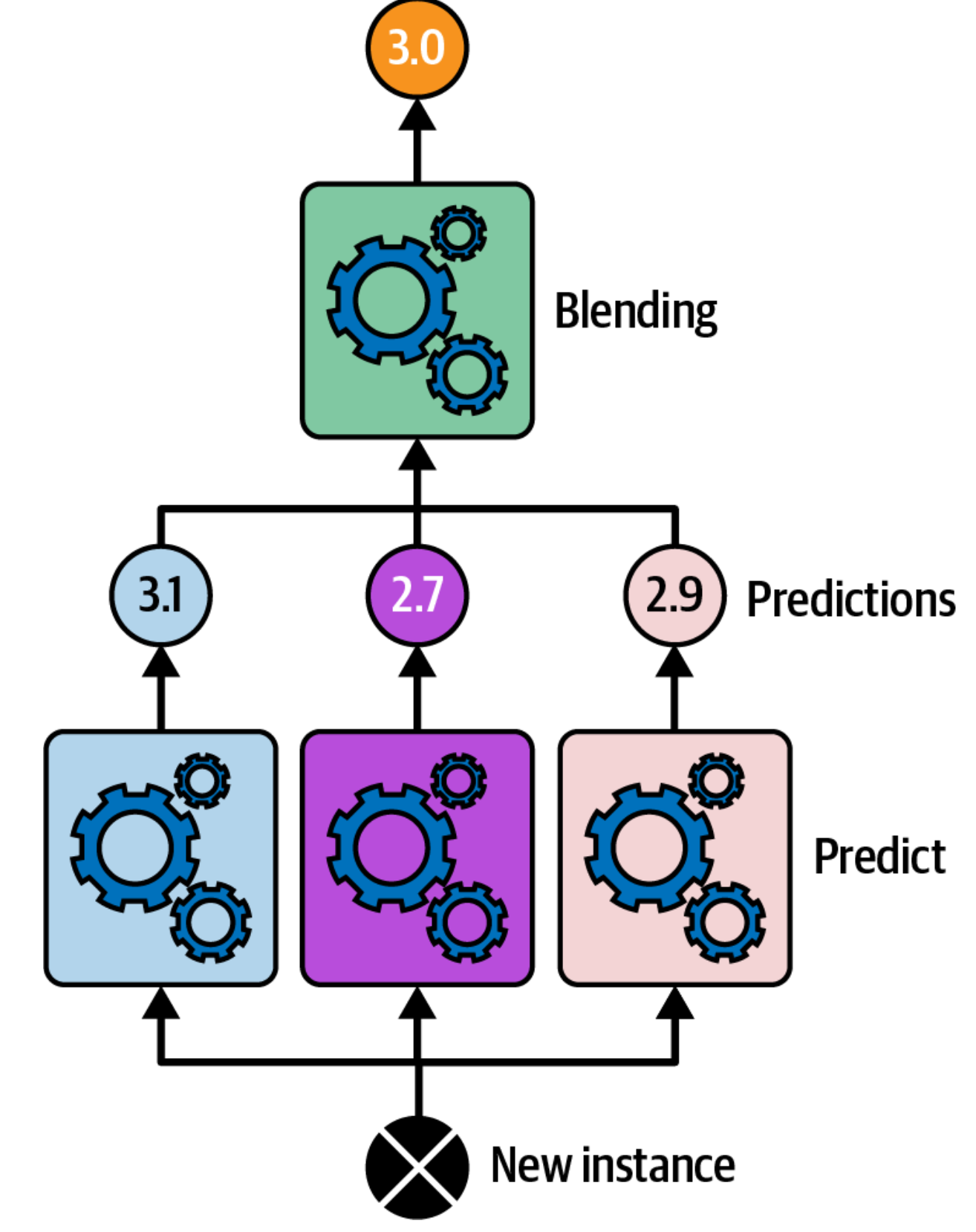
Stacking Architecture: A meta-learner (blender) learns to optimally combine predictions from multiple base models.
Building the Blending Training Set
The first step involves constructing a training set specifically for the blender model:
- Train each base model on the original training data.
- Utilize the
cross_val_predict()function to generate out-of-sample predictions for every instance in the original training data. This step is crucial as it prevents the blender from overfitting to the training set and encourages better generalization. - The resulting blending training set is formed with the following structure:
- Input features: Each instance is represented by a vector comprising the predictions from all the base models for that instance.
- Target: The target values are directly copied from the original training set.
Training the Blender
Once the blending training set is created, train the blender model on this data. The blender learns to map the input features (the base model predictions) to the target variable, essentially learning how to effectively combine the base model predictions.
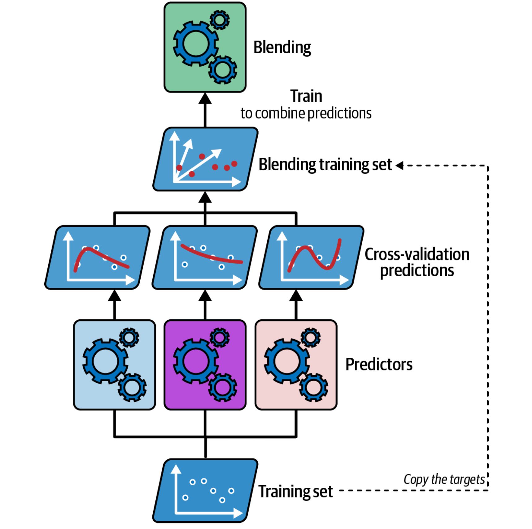
Training the Blender: The meta-learner is trained on predictions from base models to learn optimal combination weights.
Retraining Base Predictors and Making Predictions
After training the blender, retrain the base models on the complete original training data. This ensures that the base models are fully trained before making the final predictions. The prediction process for new instances involves:
- Obtaining predictions from all the base models.
- Feeding these predictions as input features to the trained blender.
- The output of the blender serves as the final ensemble prediction.
Scikit-Learn Implementation
Scikit-Learn offers convenient classes, StackingClassifier and StackingRegressor, for implementing stacking ensembles.[*](Scikit-Learn documentation: Ensemble Methods.) These classes allow you to:
- Specify the base estimators (your chosen base models).
- Select the final estimator, which is your blender model. If none is provided,
StackingClassifierusesLogisticRegression, andStackingRegressordefaults toRidgeCV. - Determine the number of cross-validation folds (
cv) used in building the blending training set.
For instance, the sources demonstrate using a StackingClassifier on the moons dataset, resulting in a slight accuracy improvement (92.8%) compared to a soft voting classifier (92%).
Multilayer Stacking and Advantages
Stacking can be extended to include multiple layers of blenders. This approach might offer additional performance gains but comes at the cost of increased training time and complexity.
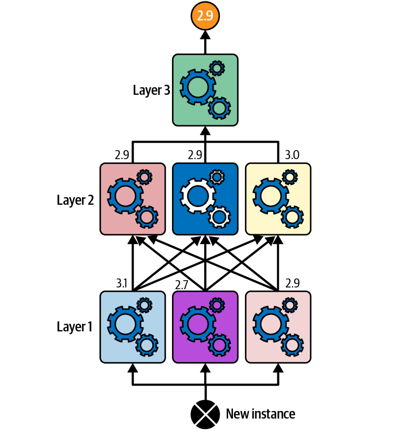
Multilayer Stacking: Multiple layers of blenders can potentially improve performance but increase complexity.
Key benefits of stacking include:
- Potential for enhanced performance: Stacking can surpass simpler ensemble methods by learning more sophisticated relationships between base model outputs and the target.
- Flexibility: You can explore various models for both the base predictors and the blender, enabling customization for specific tasks.
Key Advantages of Ensemble Learning
The sources highlight several advantages of using ensemble methods:
| Aspect | Description |
|---|---|
| Improved Accuracy | Ensemble methods often outperform individual models by combining the strengths of multiple base models and mitigating the impact of individual model errors. |
| Reduced Variance | Ensemble methods effectively reduce variance by averaging or combining predictions from multiple models, resulting in more stable and generalized predictions. |
| Robustness to Noisy Data | Ensemble methods demonstrate resilience to noisy data and outliers as the aggregation process helps to smooth out the effects of noisy data points. |
| Scalability | Many ensemble methods, such as bagging and pasting, are inherently parallelizable, making them suitable for training on large datasets. |
Conclusion
Ensemble learning represents one of the most powerful and practical approaches in machine learning, leveraging the "wisdom of the crowd" to achieve superior predictive performance. By combining multiple models through various strategies—voting, bagging, boosting, and stacking—ensemble methods effectively reduce variance, improve accuracy, and enhance robustness to noisy data.
The key to successfully applying ensemble methods lies in understanding their different approaches:
-
Voting and Bagging: Best for reducing variance when working with unstable learners like decision trees. They're parallelizable and computationally efficient.
-
Boosting: Excellent for creating strong learners from weak ones, but requires sequential training and careful hyperparameter tuning to avoid overfitting.
-
Stacking: Offers the potential for the highest performance by learning optimal combinations, but requires more computational resources and careful cross-validation to prevent overfitting.
The success of ensemble methods in machine learning competitions and real-world applications demonstrates their practical value. Whether you're building a simple voting classifier or a complex stacked ensemble, the fundamental principle remains the same: combining diverse models leads to better predictions than relying on any single model.
As machine learning continues to evolve, ensemble methods remain a cornerstone technique, providing a reliable path to high-performance models across a wide range of applications.