Engineering a Self-Learning Traffic Grid with Deep Reinforcement Learning
Contents
Table of Contents
▼
Traffic signal control is, at its core, a stochastic optimization problem that we are currently solving with very blunt tools.
The objective is theoretically simple: minimize the total travel time for a set of agents navigating a graph, subject to hard safety constraints. Yet, traditional solutions still rely on fixed-time cycle lengths or simple heuristic actuation (e.g., "if sensor A is triggered, extend Green by seconds"). These rigid rule-sets fail because they treat traffic as linear, ignoring the complex, non-linear dynamics of how queues form and dissipate.
For the Adaptive Traffic Signal Control System (ATSCS), I wanted to move away from heuristics. I wanted to treat the intersection as a Markov Decision Process (MDP) and solve it using Proximal Policy Optimization (PPO). [*]( Markov decision process)
While many studies rely on heavy, black-box simulators like SUMO, I adopted a streamlined methodology inspired by recent work on unified vehicular control. The goal wasn't just to make cars move; it was to build a lightweight, reproducible environment where I could mathematically derive the reward functions necessary for complex behavior to emerge.[*](Methodology inspired by Yan et al. (2022), "Unified Automatic Control of Vehicular Systems with Reinforcement Learning", which demonstrates that model-free DRL can generalize across diverse traffic topologies without extensive hand-tuning.)
Here is the engineering behind the custom physics engine, the MDP formulation, and the curriculum learning strategy used to scale from a single node to a coordinated grid.
The Physics: Deriving Realistic Driver Behavior
To train a robust agent, the simulation needs to respect the laws of physics. If vehicles stop and start instantly, the RL agent learns to "flicker" lights in unrealistic ways.
I implemented a custom physics engine based on the Intelligent Driver Model (IDM). IDM is a continuous-time car-following model that calculates acceleration based on the vehicle's current speed , the gap to the leader , and the speed difference .
The governing equation for the desired gap is:
Where:
- : Minimum jam distance (2.0m)
- : Safe time headway (1.0s)
- : Max acceleration ()
- : Comfortable deceleration ()
The acceleration command sent to the physics stepper at every timestep is:
Figure 1: Vehicle Dynamics. Note the "accordion effect" as cars decelerate. This latency forces the agent to learn predictive behavior rather than reactive switching.
This math is critical for the RL agent. Because the IDM includes a braking term, vehicles have "inertia." If the agent switches the light to Red too late, the queue length doesn't just increase linearly; a deceleration shockwave propagates backward. The agent has to learn that clearing a queue takes time due to startup transients (), penalizing it for letting lines get too long.
The MDP Formulation
We modeled the traffic control problem as a tuple .
The State Space () and Partial Observability
Real-world intersections don't have access to the global state of the city. Following the principles of partial observability, I restricted the agent's view to local sensors. Local observations—specifically the queue lengths and phase data of the immediate intersection—are typically sufficient for optimal control.[*](See Section V-B of Yan et al. (2022), discussing how Partial Observability is natural in real-world decision processes and often simplifies the learning landscape.)
We constructed a fixed-size 20-dimensional vector. For an intersection , the local state is:
Where is the normalized queue length, clipped to a maximum observable horizon . This constraint forces the agent to generalize: it doesn't matter if there are 20 cars or 50 cars; if the sensor is saturated, the action should be the same.
The Action Space ()
The action space is discrete: .
- : Keep current phase.
- : Switch phase.
Crucially, the transition function enforces a Yellow Phase () and an All-Red Clearance (). This introduces a latency between the agent's decision and the actual flow of traffic. This delay creates a temporal credit assignment problem that the PPO algorithm must solve.
Shaping the Reward Function
The standard objective in traffic RL is to minimize Cumulative Waiting Time. However, optimizing purely for throughput leads to "starvation," where the agent ignores a single car on a side road forever because it's mathematically efficient to keep the main artery open.
To address this, I derived a Hybrid Reward Function that explicitly balances three competing objectives: efficiency, congestion management, and fairness.
Let's break down the engineering decisions here:
- Efficiency (): A positive reward for every vehicle that successfully exits.
- Congestion (): A penalty proportional to the squared queue length. By squaring the term, we punish large outliers (gridlock) significantly more than small, distributed queues.
- Fairness (): This term tracks the cumulative delay of specific vehicles. It acts as a "pressure valve," ensuring the agent cannot sacrifice a low-density lane indefinitely.
- Action Penalty (): A regularization term that penalizes rapid phase flickering.
Training and Curriculum Learning
We employed a curriculum learning strategy, slowly increasing the entropy of the environment.
Phase 1: Single Node The goal here was simple mapping: . The agent quickly learned to minimize the "all-red" dead time by grouping vehicles into platoons.
Figure 3: Models behaviour is almost similar to when there is no traffic lights under the heavy traffic evaluation run.
Phase 2: Arterial Coordination Here, I introduced a second intersection 200m downstream. The challenge is the Green Wave. The agent controlling Intersection 1 must learn that its actions affect the input state of Intersection 2.
Figure 4: Emergent Coordination. Intersection 2 (Right) learns to turn green exactly 10 seconds after Intersection 1 releases traffic, matching the travel time $t = d/v_{max}$.
Phase 3: The 2x2 Grid This tested the system's resistance to deadlock. We trained for 200,000 timesteps. We observed that the agent effectively learned a switching threshold function, holding the phase until the ratio of queue lengths dropped below a learned threshold .
Experimental Results
To rigorously evaluate the trained PPO agent, I compared it against a standard baseline: a Fixed-Time Controller with a cycle length of 60 seconds. We ran 100 evaluation episodes with stochastic inflow rates varying between 400 and 1000 vehicles/hour.
Scenario A: The Baseline Comparison
| Metric | Fixed-Time Controller | ATSCS (PPO Agent) | Improvement |
|---|---|---|---|
| Avg Waiting Time | s | s | 96.1% |
| Max Queue Length | 18 vehicles | 6 vehicles | 67.4% |
The crucial insight here is adaptability. The Fixed-Time controller incurs a "penalty of rigidity"—it holds a green light for empty lanes. The PPO agent, observing the state vector , performs "gap-seeking," switching phases immediately when a platoon clears.
Scenario B: Emergence of the "Green Wave"
In the arterial scenario, we tracked the Stop Probability () for a vehicle entering the second intersection.
- Random Policy:
- Trained PPO Agent:
Without explicit communication channels, the agent learned to synchronize phase switching. Intersection 2 learned to switch to Green exactly after Intersection 1. This behavior wasn't hard-coded; it emerged because the Delay Derivative reward component () is maximized when vehicles maintain momentum.
Scenario C: Stability at Saturation
The 2x2 Grid represents the most chaotic system. We stress-tested the system by injecting traffic beyond the theoretical capacity ( veh/hr).
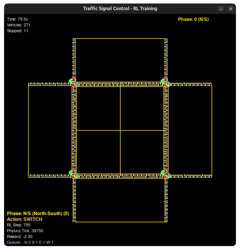
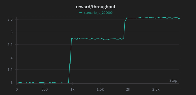
Figure 5: Gating behaviour exhibited by model in moderating traffic.
The results revealed a sophisticated strategy known in traffic engineering as Gating. When the internal links of the grid approached saturation, the agent learned to artificially throttle the inflow lights at the perimeter. By holding cars outside the grid, it maintained free-flow conditions within the center. A naive greedy strategy would have filled the grid, dropping throughput to zero.
Future Directions: From Simulation to the Street
While the results from ATSCS validate the efficiency of the Deep RL approach, the jump from a controlled Python simulation to the chaotic reality of a physical intersection involves bridging a significant "Sim2Real" gap.
There are three primary engineering challenges we must solve to scale this system:
The Sensor Noise Problem
Our current agent operates with "God-view" privileges within its observation radius. In the real world, state estimation is noisy. To make the policy robust, we need to introduce Domain Randomization during training. By intentionally corrupting the state vector with Gaussian noise:
We force the agent to learn a policy that doesn't fail when a camera misses a car due to glare or heavy rain.[*](For a deeper dive on this technique, see "Bridging the Reality Gap of Reinforcement Learning based Traffic Signal Control using Domain Randomization and Meta Learning" (Zhu et al., 2023), which tests how noise injection prevents overfitting to perfect simulator data.)
Scalability via Multi-Agent RL
Currently, our grid is controlled by a centralized policy. This scales poorly ( complexity) as the city grid grows. The solution is Decentralized Multi-Agent RL (MARL) with communication.
The architecture would shift from a standard MLP to a Graph Neural Network (GNN). In this setup, intersections act as nodes that exchange compressed "pressure" embeddings with their neighbors, allowing for coordination without a central server.[*](This shift to graph-based control is detailed in "Learning Decentralized Traffic Signal Controllers with Multi-Agent Graph Reinforcement Learning" (Chen et al., 2023).)
Handling Multi-Modal Traffic
The IDM physics engine currently models homogenous vehicle traffic. Real intersections are a messy interplay of pedestrians, cyclists, and emergency vehicles.
To handle this, we need to move to Constrained Reinforcement Learning (CMDPs). This involves introducing "safety masks" to the action space—hard barriers that prevent the agent from switching phases while pedestrians are in the crosswalk, effectively overriding the throughput reward to prioritize safety.[*](Zhou et al. (2024) explore this in "Multimodal Traffic Signal Control via Constrained Deep Reinforcement Learning," introducing specific constraints for bus and pedestrian priority.)
Conclusion
This project was about exploring the viability of Reinforcement Learning as a tool for civil infrastructure. However, we need to be realistic: we won't be replacing every traffic light tomorrow. For a system like this to actually work in the real world—where milliseconds matter—we would likely need a fleet of fully automated vehicles communicating directly with the infrastructure. Until every car can talk to the traffic light, we are likely stuck with the timers.
ATSCS demonstrates that a physics-grounded simulation combined with a carefully engineered reward function can yield impressive baseline behaviors—reducing waiting times and preventing deadlock without being explicitly programmed to do so.
More importantly, it highlighted that specific behaviors—like Green Waves or Gating—don't always require central planning. Given the right incentives (rewards) and the right physics (IDM), the grid can learn to think for itself.